hello, i dont know why stata keeps me showing invalid syntax in this loop:
foreach x of p524a1_14 p524a1_15 p524a1_16 p524a1_17 p524a1_18{
summ `x'
gen ING_`x' = (`x'-r(mean))/r(sd)
}
i tried with an space just before the "{" and every way but i cant do it
please send your suggestion
thank you so much
Thursday, September 30, 2021
Survival Analysis - different outputs
Hello everyone,
I am trying to do survival analysis on 2018 Nigeria Demographic and Health Survey Data.
The data has 33,924 observations, but after I expanded it to capture every month a child lived before death or censoring it got to 934,141 observations.
From what I understand from texts, 'sts list' and 'ltable t dead, noadjust' commands should give the same output.
But I'm getting different outputs:
'sts list' used 33,924 as its beginning total and at the end of the 60-month period, there are 88.28 percent children still alive, which looks about right. While,
'ltable t dead, noadjust' used 934,141 as its beginning total and at the end of the 60-month period, there are 99.39 children still alive.
Please, I want to understand what could be wrong, since both outputs should be the same.
What did I do wrong please?
Below is the dataex output
Thank you for your help.
I am trying to do survival analysis on 2018 Nigeria Demographic and Health Survey Data.
The data has 33,924 observations, but after I expanded it to capture every month a child lived before death or censoring it got to 934,141 observations.
From what I understand from texts, 'sts list' and 'ltable t dead, noadjust' commands should give the same output.
But I'm getting different outputs:
'sts list' used 33,924 as its beginning total and at the end of the 60-month period, there are 88.28 percent children still alive, which looks about right. While,
'ltable t dead, noadjust' used 934,141 as its beginning total and at the end of the 60-month period, there are 99.39 children still alive.
Please, I want to understand what could be wrong, since both outputs should be the same.
What did I do wrong please?
Below is the dataex output
Code:
* Example generated by -dataex-. To install: ssc install dataex
clear
input float(t pid study_time) byte died float dead
 1 1 13 0 0
 2 1 13 0 0
 3 1 13 0 0
 4 1 13 0 0
 5 1 13 0 0
 6 1 13 0 0
 7 1 13 0 0
 8 1 13 0 0
 9 1 13 0 0
10 1 13 0 0
11 1 13 0 0
12 1 13 0 0
13 1 13 0 0
 1 2  9 0 0
 2 2  9 0 0
 3 2  9 0 0
 4 2  9 0 0
 5 2  9 0 0
 6 2  9 0 0
 7 2  9 0 0
 8 2  9 0 0
 9 2  9 0 0
 1 3 17 0 0
 2 3 17 0 0
 3 3 17 0 0
 4 3 17 0 0
 5 3 17 0 0
 6 3 17 0 0
 7 3 17 0 0
 8 3 17 0 0
 9 3 17 0 0
10 3 17 0 0
11 3 17 0 0
12 3 17 0 0
13 3 17 0 0
14 3 17 0 0
15 3 17 0 0
16 3 17 0 0
17 3 17 0 0
 1 4 31 0 0
 2 4 31 0 0
 3 4 31 0 0
 4 4 31 0 0
 5 4 31 0 0
 6 4 31 0 0
 7 4 31 0 0
 8 4 31 0 0
 9 4 31 0 0
10 4 31 0 0
11 4 31 0 0
12 4 31 0 0
13 4 31 0 0
14 4 31 0 0
15 4 31 0 0
16 4 31 0 0
17 4 31 0 0
18 4 31 0 0
19 4 31 0 0
20 4 31 0 0
21 4 31 0 0
22 4 31 0 0
23 4 31 0 0
24 4 31 0 0
25 4 31 0 0
26 4 31 0 0
27 4 31 0 0
28 4 31 0 0
29 4 31 0 0
30 4 31 0 0
31 4 31 0 0
 1 5 39 0 0
 2 5 39 0 0
 3 5 39 0 0
 4 5 39 0 0
 5 5 39 0 0
 6 5 39 0 0
 7 5 39 0 0
 8 5 39 0 0
 9 5 39 0 0
10 5 39 0 0
11 5 39 0 0
12 5 39 0 0
13 5 39 0 0
14 5 39 0 0
15 5 39 0 0
16 5 39 0 0
17 5 39 0 0
18 5 39 0 0
19 5 39 0 0
20 5 39 0 0
21 5 39 0 0
22 5 39 0 0
23 5 39 0 0
24 5 39 0 0
25 5 39 0 0
26 5 39 0 0
27 5 39 0 0
28 5 39 0 0
29 5 39 0 0
30 5 39 0 0
end
Thank you for your help.
Arranging bars of graph bar
Hello community. I am producing a graph with Stata. Here is the output :
Array
And here is the code
I would rather like to put the bars of the same color side-by-side. So three groups (Av. var1 for the two groups of Catvar), (Av. var2 for the two groups of Catvar), and (Av. var3 for the two groups of Catvar). This is possible in Excel for example. Is it possible with Stata ? Any help is welcome.
Best.
Array
And here is the code
Code:
graph bar var1 var2 var3 [aw=weight], ///
over(Catvar) ///
blabel(bar,format(%9.2f)) ///
legend(label(1 "Av. var1") label(2 "Av. var2") ///
label(3 "Avg 3")) yla(5(5)25,nogrid) graphregion(color(white))
Best.
Reshape numerous variables
I have a vector of numerous variables (>100) that I need to reshape. Basically the format of the variables are the following.
Country GDP Population v1_2000 v1_2001 v1_2002 .. v1_2020 v2_2000 v2_2001 v2_2002 ... v2_2020 .... v50_2000 v50_2001 ... v50_2020
For the simplicity I generated data as suggested.
Then of course, here I have only two variables (v1_, v2_), so I can simply do
But in my actual data, I have v1_, v2_, ...... v_100.
I tried to define
and etc, but so far nothing works.
How can we reshape such large list of variables v1_, ..... v100_ ?
Country GDP Population v1_2000 v1_2001 v1_2002 .. v1_2020 v2_2000 v2_2001 v2_2002 ... v2_2020 .... v50_2000 v50_2001 ... v50_2020
For the simplicity I generated data as suggested.
Code:
clear
    input str72 country str24 units float(v1_2000 v1_2001 v1_2002 v1_2003) double(v2_2000 v2_2001  v2_2002 v2_2003)
    "Austria" "Percent change" 2.048 -3.613 1.329 1.708 1.806 1.999 2.086 2.197
    "Austria" "Percent of potential GDP" -1.804 -2.958 -4.279 -4.092 . . . .
    "Belgium" "Percent change" .832 -3.006 1.153 1.336 1.605 1.707 1.83 1.876
    "Belgium" "Percent of potential GDP" -2.112 -4.786 -4.257 -3.425 . . . .
    "Czech Republic" "Percent change" 2.464 -4.287 1.675 2.629 3.5 3.5 3.5 3.5
    "Czech Republic" "Percent of potential GDP" . . . . . . . .
    "Denmark" "Percent change" -.87 -5.071 1.2 1.557 2.567 2.634 2.297 2.344
    "Denmark" "Percent of potential GDP" 3.692 .038 -1.726 -1.494 . . . .
endCode:
reshape long v1_ v2_ , i(country units) j(year)
I tried to define
Code:
local varlist v1_ v2_ ... v_100
How can we reshape such large list of variables v1_, ..... v100_ ?
Stratified sample with probability proportional to size
We have a total of 908 communities (each community has a number of households) which are located in the sphere of influence of roads / highways (social inclusion and logistics corridors), they are divided into groups (intervention and control) and They belong to 2 strata: near and far (with respect to the capital of the community). A community should be selected with a probability proportional to the number of households in each community within each strata, each type of road / highway and group to which it belongs. What command in Stata could be used to make the community selection with PPS?
Combining Two Similar Variables To be in one row
Hi All,
I have the following 2 variables that serve the same purpose and I'm trying to generate one variable for both. Schoolfees1 has school values for ages 15 years to 19 years. Schoolfees2 is school values for ages 10 to 14 year olds. I would like to generate an overall fees variable called fees1 and would like the amount of school fees to show. The results shows as 0 or 1.
*My results show as follows
*Please note that gap are other ages that are not part of the equation. I'm only interested in ages 10 to 19 year old
input long(schoolfees1 schoolfees2) float fees1
. . .
. . .
. . .
. . .
. . .
. . .
. . .
. . .
. . .
7500 . 1
. . .
. . .
. . .
. . .
. . .
. . .
. . .
. . .
. . .
. . .
. . .
. . .
. . .
. . .
. . .
. . .
. . .
. . .
700 . 1
. . .
. . .
. . .
. . .
. . .
. . .
. . .
4000 . 1
. . .
. . .
. . .
. . .
. . .
. . .
. . .
. . .
. . .
250 . .
100 . 1
15 . 1
. . .
250 . 1
. . .
. . .
. . .
. . .
. . .
. . .
50 . 1
. . .
. . .
. . .
. . .
. . .
. . .
. . .
. . .
. . .
. . .
. . .
. . .
. . .
. . .
. . .
. . .
. . .
. . 1
. . .
. . .
. . .
650 . 1
. . .
. . .
. . .
. . .
. . 1
. . .
. . .
. . .
. . .
. . .
. . .
. . .
. . .
. . .
. . .
. . .
. . .
. . .
650 . 1
. . .
end
label values schoolfees1 w1_nonres
label values schoolfees2 w1_nonres
[/CODE]
Thanks
Nthato
I have the following 2 variables that serve the same purpose and I'm trying to generate one variable for both. Schoolfees1 has school values for ages 15 years to 19 years. Schoolfees2 is school values for ages 10 to 14 year olds. I would like to generate an overall fees variable called fees1 and would like the amount of school fees to show. The results shows as 0 or 1.
Code:
gen fees1 = schoolfees1 | schoolfees2 if age1>9 & age1<20
*Please note that gap are other ages that are not part of the equation. I'm only interested in ages 10 to 19 year old
input long(schoolfees1 schoolfees2) float fees1
. . .
. . .
. . .
. . .
. . .
. . .
. . .
. . .
. . .
7500 . 1
. . .
. . .
. . .
. . .
. . .
. . .
. . .
. . .
. . .
. . .
. . .
. . .
. . .
. . .
. . .
. . .
. . .
. . .
700 . 1
. . .
. . .
. . .
. . .
. . .
. . .
. . .
4000 . 1
. . .
. . .
. . .
. . .
. . .
. . .
. . .
. . .
. . .
250 . .
100 . 1
15 . 1
. . .
250 . 1
. . .
. . .
. . .
. . .
. . .
. . .
50 . 1
. . .
. . .
. . .
. . .
. . .
. . .
. . .
. . .
. . .
. . .
. . .
. . .
. . .
. . .
. . .
. . .
. . .
. . 1
. . .
. . .
. . .
650 . 1
. . .
. . .
. . .
. . .
. . 1
. . .
. . .
. . .
. . .
. . .
. . .
. . .
. . .
. . .
. . .
. . .
. . .
. . .
650 . 1
. . .
end
label values schoolfees1 w1_nonres
label values schoolfees2 w1_nonres
[/CODE]
Thanks
Nthato
quarterly returns
Hi
To calculate quarterly index returns from monthly index returns starting from the first month of the quarter to the third month of the quarter, I do:
I want now to calculate quarterly index returns starting from one month prior to the quarter-end until two months after the quarter-end. How can I adjust my code to achieve this?
An example of my data is here:
Thanks
To calculate quarterly index returns from monthly index returns starting from the first month of the quarter to the third month of the quarter, I do:
Code:
gen log_monthly_factor=log(1+vwretd)
by fqdate, sort: egen quarterly_vwretd=total(log_monthly_factor)
replace quarterly_vwretd=(exp(quarterly_vwretd)-1)
An example of my data is here:
Code:
* Example generated by -dataex-. To install: ssc install dataex
clear
input long DATE double vwretd float(year fqdate)
  28            -.06624392 1960  0
  59             .01441908 1960  0
  90            -.01282217 1960  0
 119            -.01527067 1960  1
 151             .03409799 1960  1
 181              .0228328 1960  1
 210            -.02270468 1960  2
 243             .03221498 1960  2
 273  -.058673340000000004 1960  2
 304           -.004704664 1960  3
 334              .0486173 1960  3
 364             .04853724 1960  3
 396              .0639524 1961  4
 424             .03700465 1961  4
 454   .030609920000000002 1961  4
 483   .005644733000000001 1961  5
 516             .02589407 1961  5
 546            -.02849906 1961  5
 577             .02995465 1961  6
 608   .026854410000000002 1961  6
 637            -.01999036 1961  6
 669   .027331130000000002 1961  7
 699             .04545113 1961  7
 728           .0007129512 1961  7
 761  -.036146990000000004 1962  8
 789             .01951236 1962  8
end
format %td DATE
format %tq fqdate
The "replace" option to the table command in Stata 16 is on longer available in Stata17; is there an alternative in Stata 17?
In Stata 16 you could code:
table ..., replace
to replace the data in memory with the results produced by the table command.
Is there an alternative in Stata 17, or a way to convert results from a collection to data?
Regards Kim
table ..., replace
to replace the data in memory with the results produced by the table command.
Is there an alternative in Stata 17, or a way to convert results from a collection to data?
Regards Kim
Kleibergen Paap F statistic test in xtdpdgmm
Hi everyone, I'm currently working with xtdpdgmm for my thesis but I'm confused how to get Kleibergen Paap F statistic test for weak instrument, can someone help me?
Here 's my code :
xtdpdgmm ROA l.DebtTA bi_3thn_out gsales size c.size#c.size c.l.DebtTA#c.bi_3thn_out if tin(2009,2019), model(diff) gmm(bi_3thn_out, lag(2 4) m(level)) gmm(ndtax tan, lag(2 2) diff m(diff)) two vce(r) nofootnote
Thankyou in advance!
Here 's my code :
xtdpdgmm ROA l.DebtTA bi_3thn_out gsales size c.size#c.size c.l.DebtTA#c.bi_3thn_out if tin(2009,2019), model(diff) gmm(bi_3thn_out, lag(2 4) m(level)) gmm(ndtax tan, lag(2 2) diff m(diff)) two vce(r) nofootnote
Thankyou in advance!
how to do instrument strength test for non-i.i.d error (more than one endogenous variables)
Dear all,
I wish to test instrument strength for the non-i.i.d error, and I have 3 endogenous variables. I noticed that the STATA command weakivtest by Montiel Olea and Pflueger (2013) is robust to non-i.i.d error, but it is restricted to one endogenous variable. Is there any code or literature suggested regarding multiple endogenous variables?
Great thanks,
Haiyan
How do I create a new variable which counts number of variables that satisfy a given condition?
Hallo Statalist,
I am new here. I have a dataset of different towns with monthly temperatures over a 10-year period (i.e. 120 months). The dataset has just over 16,000 towns. I want a new variable which gives me the number of times each town recorded temperature exceeding a given threshold, say 15 degrees. Is there a simple was to do this without reshaping the data? Here is the sample data for the first 5 towns over the first 5 months
Thanks you!
I am new here. I have a dataset of different towns with monthly temperatures over a 10-year period (i.e. 120 months). The dataset has just over 16,000 towns. I want a new variable which gives me the number of times each town recorded temperature exceeding a given threshold, say 15 degrees. Is there a simple was to do this without reshaping the data? Here is the sample data for the first 5 towns over the first 5 months
Code:
     +------------------------------------------------------+
     | town_id   month1   month2   month3   month4   month5 |
     |------------------------------------------------------|
  1. |       1       17       10       28        4        6 |
  2. |       2       14       29       15       20       16 |
  3. |       3       26        7        4        5        7 |
  4. |       4       25        6       29       13       10 |
  5. |       5        6       17        7        5       24 |
+------------------------------------------------------+create v3 which shows number of v1 that share the same v2 value
Hi,
My dataset has 2 variables that I am interested in seeing the relationship between.
v1 is 'unique_attend' which creates a unique code for each attendance (regardless of how many occur on the same day, or years apart etc.)
v2 is 'ID' which creates a unique ID number that is assigned to an individual.
Thus if there are 5 'unique_attend' cases with the same 'ID', that person has attended 5 times.
I want to create a third variable 'num_attend' which would show how many attendances are associated with each ID, but I can't for the life of me think of how to write that condition, and haven't been able to yield anything through searching.
Thanks in advance for the help,
Jane.
coefplot plotting results from categorical variable
Dear all,
I would like to use coefplot to compare the coefficients from different models and categorical variables. I am using different data, but I recreated a (nonsensical) example that shows my question using the auto-dataset:
My issue with the graph is that there are two groups (1.dummy_weight and 2.dummy_weight) and for each of them est_1 and est_2 are presented separately. Is there a way to have only est_1 and est_2 once on the y-axis, and then compare 1.dummy_weight and 2_dummy_weight next to it? So that there is not est_1 and est_2 in the legend at the bottom, but 1.dummy_weight and 2.dummy_weight (in blue and red)?
I am attaching a screenshot from the output and what I would like to have.
Thank you very much for your help!
All the best
Leon
Array
I would like to use coefplot to compare the coefficients from different models and categorical variables. I am using different data, but I recreated a (nonsensical) example that shows my question using the auto-dataset:
Code:
webuse auto, clear
gen dummy_weight = 0 // I define a categorical variable for the weight of a car
replace dummy_weight = 1 if weight > 2000 & weight <= 3000
replace dummy_weight = 2 if weight > 3000
eststo est_1: reg headroom i.dummy_weight if foreign == 0 // I estimate a model separate for domestic and foreign car makers
eststo est_2: reg headroom i.dummy_weight if foreign == 1
coefplot est_*, keep(1.dummy_weight 2.dummy_weight) swapnames asequation // I compare the coefficents
I am attaching a screenshot from the output and what I would like to have.
Thank you very much for your help!
All the best
Leon
Array
Wednesday, September 29, 2021
Labels of restricted categories appearing in graph when using -by()-
I want to graph tobacco use for couples in different value groups. While the values variable has 12 categories, I only want to graph the first five, and I use -inrange()- to achieve that:
Array
However, when I add the line of code with -by()- (below), the restriction imposed by -inrange(values, 1, 5) no longer holds and the labels for all the categories appear in the graph. How can I limit this to the first five categories (G1 to G5) as shown in the first figure?
Note: "at3" is a dummy variable with values 0/1. (As an aside, how can I relabel the variable in -by()- as done with -over()-?).
Array
Stata v.15.1. Using panel data.
Code:
graph hbar lstbcn1 lstbcn2 if inrange(values, 1, 5) , nooutsides  ///
bar(1, bfcolor(navy)) bar(2, bfcolor(maroon)) over(values, label(labsize(small))  ///
relabel(1 "G1" 2 "G2" 3 "G3" 4 "G4" 5 "G5")) ///
ti("", size(small)) ylabel(, labsize(small)) ytick(25(50)175, grid) ///
legend(region(lstyle(none)) order(1 "male" 2 "female") ///
rowgap(.1) colgap(1) size(small) color(none) region(fcolor(none))) name(c1, replace) ///
graphregion(margin(medthin) color(white) icolor(white)) plotregion(style(none) color(white) icolor(white))However, when I add the line of code with -by()- (below), the restriction imposed by -inrange(values, 1, 5) no longer holds and the labels for all the categories appear in the graph. How can I limit this to the first five categories (G1 to G5) as shown in the first figure?
Code:
by(at3, note("") graphregion(color(white))) ///Array
Code:
* Example generated by -dataex-. To install: ssc install dataex
clear
input int(lstbcn1 lstbcn2) byte(values at3)
 50  60 1 0
100  50 2 0
140 200 3 0
  8  25 4 1
 20   4 5 1
 10  60 2 1
 50 110 7 0
 75 100 1 0
 50  35 2 0
  8  25 3 1
 20   4 5 1
125 100 3 0
 80  25 4 0
140  60 5 0
 40  20 5 1
 60  40 6 0
  6   2 5 1
  8  25 3 1
 20   4 2 1
100 100 1 0
  7   5 2 1
 35   2 3 1
  7   5 4 1
 35   2 4 1
 60  30 2 1
  6   2 5 1
100 100 5 0
  7   5 5 1
 35   2 5 1
150 100 6 0
140  28 7 0
 15  10 6 1
 14   8 7 1
 30 160 7 1
 70  70 4 0
 50  10 4 0
 25  35 3 1
 60  30 3 0
250 140 2 0
100 140 2 0
 50  80 2 1
end
What fixed effects I should add when using triple difference in firm level?
In my difference-in-difference setting (double diff), I examine the impact of anticorruption laws on firms' asset growth of all countries all over the world after the laws are implemented in each country.
I normally control for firm and industry * year fixed effects in this case following existing literature.
However, I reckon that the impacts of laws will be different between developed and developing countries. Therefore, I am thinking of using subsample tests. There are two ways of conducting a subsample test are 1) divide the whole sample into two subsamples and then run the main regression for all subsamples or (2) add the interaction for one subsample and see the difference by reading the interactive coefficients by running the regression.
Regarding the method (2) in double diff, we call it diff-in-diff-in-diff or triple diff. And (2) is preferred compared to (1).
So, what I want to ask is, if in the main specification, I control for firm and industry * year fix effects, so what fixed effects I should control when I perform the triple diff to examine the additional impact of laws on developed countries?
I normally control for firm and industry * year fixed effects in this case following existing literature.
However, I reckon that the impacts of laws will be different between developed and developing countries. Therefore, I am thinking of using subsample tests. There are two ways of conducting a subsample test are
1) divide the whole sample into two subsamples and then run the main regression for all subsamples or (2) add the interaction for one subsample and see the difference by reading the interactive coefficients by running the regression.Regarding the method (2) in double diff, we call it diff-in-diff-in-diff or triple diff. And (2) is preferred compared to (1).
So, what I want to ask is, if in the main specification, I control for firm and industry * year fix effects, so what fixed effects I should control when I perform the triple diff to examine the additional impact of laws on developed countries?
Square CSR: a brief overview
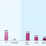 Square CSR programs and initiatives mainly focus on four key priority areas – Climate Action, Social Impact, Employees and Culture, and Corporate Governance. These initiatives are led by Neil Jorgensen, Global Environmental, Social, and Governance Lead at Square. Square Supporting Local Communities Square has invested USD 100 million in minority and underserved communities The financial unicorn assists some local communities in the US to preserve their local culture and deal with other most pressing issues. In many offices there are active volunteer communities, referred to volunteams that undertake various projects to support local communities Square and Gender Equality and Minorities Square invests in employee resource groups such as Black Squares Association, LatinX Community, LGBTQ group, and others in order to create an inclusive environment The majority 54,1% of US employees of The fintech are white people, as illustrated in Figure 1 below: Figure 1 Race and ethnicity of Square Inc. employees in US[1] Energy Consumption by Square Square launched Bitcoin Clean Energy Investment Initiative, USD 10 million investment to help accelerate renewable energy adoption in bitcoin mining. The payments company is planning to evaluate and explore clean energy options, working closely with its key provider partners. Carbon Emissions by Square In 2020 the total carbon footprint for Square totalled to 247,900 tCO2e. The Figure 2 below illustrates the share of carbon emissions by operations: Figure 2 Square Inc. total carbon emissions in 2020[2] The financial services and digital payments company has aimed to be zero carbon for operations by 2030. Other CSR Initiatives and Charitable Donations by Square Leads Program offered to managers at all levels is designed to develop leadership skills and competencies The finance sector disruptor fully pays parental leave globally, caregiving leave to US employees In UK Square partnered with The Entrepreneurial…
Is there any package for stacked event-by-event estimates ?
I am reading a paper of Cengiz, 2019 about using stacked event-by-event estimates for the Difference-in-Differences settings. This is a good estimator for examining the effect of law without any control unit.I am wondering if Stata has any package for this estimator.
Many thanks and warm regards.
Many thanks and warm regards.
What is the difference between "stack" and "pca" ?
From my understanding, it seems that pca and stack syntaxes are all about suppressing two or more variables (similar characteristics) to one variable. Is there any difference between these two?
Trying to open shapefile but Stata looks for .dbf file
Hello,
I am trying to open a shapefile under the name "pga.shp" that I downloaded from the US Geological Survey. I am using shp2dta in Stata/MP 16.0.
This is the line of code I am using
When I run this, I get the following error:
I am puzzled as to why Stata is looking for a .dbf file when the one it should open is a .shp file. I do not have the .dbf files by the way. Just .shp
Any help would be appreciated.
Michelle Escobar
I am trying to open a shapefile under the name "pga.shp" that I downloaded from the US Geological Survey. I am using shp2dta in Stata/MP 16.0.
This is the line of code I am using
Code:
shp2dta using pga.shp, data(pga_data) coor(pga_coordinates) genid(id)
Code:
file pga.dbf not found
r(601);
Any help would be appreciated.
Michelle Escobar
2SLS: Interpretation of Results
Hi - I am working with panel data (US industrials, 2000-2019) and am researching the impact of firm geographic diversification (GSD) on firm performance (ROA.) Fixed effects repression suggests an inverted U relationship between GSD and ROA. The linear and quadratic relationship of GSD performance are both significant. As a robustness check, I used 2SLS to correct for endogeneity of the regressor GSD (linear and quadratic.) The post estimation tests suggested that underidentification, weak identification annd over identification were not a problem and the regressor did in fact have an endogeneity issue. However, the results of 2SLS suggest non-significant relationship between GSD and performance. I am wondering how to interpret this result. In case you have any suggestions, please do let me know. Thank you.
Code:
. xtivreg2 Ln_EBIT_ROA Ln_Revenue Ln_LTD_to_Sales Ln_Intangible_Assets CoAge wGDPpc wCPI wDCF w
> Expgr wGDPgr wCons Ln_PS_RD (l1.Ln_GSD l1.Ln_GSD_Sqd= l1.Ln_Indgrp_GSD_by_Year Ln_Int_exp Ln_
> Int_exp_Sqd l1.Ln_ROS) if CoAge>=0 & NATION=="UNITED STATES" & NATIONCODE==840 & FSTS>=10 & G
> ENERALINDUSTRYCLASSIFICATION ==1 & Year_<2020 & Year_<YearInactive & Discr_GS_Rev!=1, fe endo
> g (l1.Ln_GSD)
Warning - singleton groups detected.  35 observation(s) not used.

FIXED EFFECTS ESTIMATION
------------------------
Number of groups =       141                    Obs per group: min =         2
                                                               avg =       5.7
                                                               max =        17

IV (2SLS) estimation
--------------------

Estimates efficient for homoskedasticity only
Statistics consistent for homoskedasticity only

                                                      Number of obs =      798
                                                      F( 13,   644) =     4.41
                                                      Prob > F      =   0.0000
Total (centered) SS     =  203.9428465                Centered R2   =  -0.0686
Total (uncentered) SS   =  203.9428465                Uncentered R2 =  -0.0686
Residual SS             =  217.9269693                Root MSE      =    .5759

--------------------------------------------------------------------------------------
         Ln_EBIT_ROA |      Coef.   Std. Err.      z    P>|z|     [95% Conf. Interval]
---------------------+----------------------------------------------------------------
              Ln_GSD |
                 L1. |  -.7524867   .4739275    -1.59   0.112    -1.681367    .1763941
                     |
          Ln_GSD_Sqd |
                 L1. |    .108648   .1192194     0.91   0.362    -.1250177    .3423138
                     |
          Ln_Revenue |   .5130579   .1374392     3.73   0.000      .243682    .7824338
     Ln_LTD_to_Sales |  -.1517859   .0352142    -4.31   0.000    -.2208044   -.0827674
Ln_Intangible_Assets |  -.0811832     .04624    -1.76   0.079    -.1718119    .0094456
               CoAge |  -.0249093   .0143349    -1.74   0.082    -.0530053    .0031866
              wGDPpc |   .0000639   .0000309     2.07   0.039     3.33e-06    .0001244
                wCPI |  -.0016804   .0280792    -0.06   0.952    -.0567146    .0533538
                wDCF |  -2.80e-15   1.67e-13    -0.02   0.987    -3.29e-13    3.24e-13
              wExpgr |   .0132025   .0114394     1.15   0.248    -.0092182    .0356232
              wGDPgr |  -.0291117   .0338202    -0.86   0.389    -.0953981    .0371747
               wCons |   2.88e-14   6.23e-14     0.46   0.644    -9.32e-14    1.51e-13
            Ln_PS_RD |  -.0570622   .0723795    -0.79   0.430    -.1989234     .084799
--------------------------------------------------------------------------------------
Underidentification test (Anderson canon. corr. LM statistic):          45.779
                                                   Chi-sq(3) P-val =    0.0000
------------------------------------------------------------------------------
Weak identification test (Cragg-Donald Wald F statistic):               12.021
Stock-Yogo weak ID test critical values:  5% maximal IV relative bias    11.04
                                         10% maximal IV relative bias     7.56
                                         20% maximal IV relative bias     5.57
                                         30% maximal IV relative bias     4.73
                                         10% maximal IV size             16.87
                                         15% maximal IV size              9.93
                                         20% maximal IV size              7.54
                                         25% maximal IV size              6.28
Source: Stock-Yogo (2005).  Reproduced by permission.
------------------------------------------------------------------------------
Sargan statistic (overidentification test of all instruments):           2.186
                                                   Chi-sq(2) P-val =    0.3352
-endog- option:
Endogeneity test of endogenous regressors:                               8.598
                                                   Chi-sq(1) P-val =    0.0034
Regressors tested:    L.Ln_GSD
------------------------------------------------------------------------------
Instrumented:         L.Ln_GSD L.Ln_GSD_Sqd
Included instruments: Ln_Revenue Ln_LTD_to_Sales Ln_Intangible_Assets CoAge
                      wGDPpc wCPI wDCF wExpgr wGDPgr wCons Ln_PS_RD
Excluded instruments: L.Ln_Indgrp_GSD_by_Year Ln_Int_exp Ln_Int_exp_Sqd
                      L.Ln_ROS
------------------------------------------------------------------------------How to list all unique values based on value of another variable?
Hi all, I am conducting a cross-country analysis.
I have a variable named developed has the value of 1 if this country is a developed country and 0 otherwise. Now I want to list all developed countries (variable's name is country) where developed=1, can I ask what I should do then?
Many thanks and warm regards.
I have a variable named developed has the value of 1 if this country is a developed country and 0 otherwise. Now I want to list all developed countries (variable's name is country) where developed=1, can I ask what I should do then?
Many thanks and warm regards.
Square Ecosystem: a brief overview
 Square ecosystem represents a growing ecosystem of financial services. Ecosystem of Square can be divided into two groups: seller ecosystem and cash ecosystem. Square seller ecosystem is a cohesive commerce ecosystem that helps its sellers start, run, and grow their businesses. As illustrated in Figure 1 below, the core services for sellers are managed payments and points of sales products and services. Specific functionalities that contribute to these services include customer engagement platform, payroll invoices services, functionality to make appointments and capital management tools. Moreover, e-commerce and developer platforms, as well as, virtual terminal are important components of Square ecosystem on the Seller front. Figure 1 Square Seller products and services Square cash ecosystem, represented by Cash App comprises a wide range of financial products and services that are designed to help individuals manage their money. These include a cash card, instant discounts tool Boost. The strongest feature of Cash App that has no analogue in the market is the functionality to purchase Bitcoints and stocks in a simple, secure and hassle-free manner. Figure 2 Square Cash App functionalities The financial services and digital payments company is increasing the linkage between its seller and cash ecosystem in order to from strengthen its position in the market. For example, employers with seller account can pay their employees from seller revenues the next business day using Instant Payments feature when employees use Cash App. There is still room for growth of Square ecosystem on both fronts – Seller and Cash App. Apart from connecting the both ecosystems. The finance sector disruptor can also scale each of them, as well as, engage in optimised cross-selling. Moreover, the developer platform can play an instrumental role in expanding the ecosystem for Square, through exposing Application Program Interface (API) to third party developers to adjust it…
Square McKinsey 7S Model
 Square McKinsey 7S model is intended to illustrate how seven elements of business can be aligned to increase effectiveness. The framework divides business elements into two groups – hard and soft. Strategy, structure and systems are considered hard elements, whereas shared values, skills, style and staff are soft elements. According to Square McKinsey 7S model, there is a strong link between elements and a change in one element causes changes in others. Moreover, shared values are the most important of elements because they cause influence other elements to a great extent. McKinsey 7S model Hard Elements in Square McKinsey 7S Model Strategy Square business strategy is based on principles of simplifying financial transactions and developing an ecosystem of financial products and services. The financial services platform has two types of ecosystem – seller ecosystem and cash ecosystem. Square systematically expands both ecosystems with addition of new financial products and services that simplify processes and challenge the status quo. Structure Square organizational structure is highly dynamic, reflecting the rapid expansion of the range of financial products and services offered by the finance sector disruptor. Although it is difficult to frame Square organizational culture into any category due to the complexity of the business, it is closer to flat organizational structure compared to known alternatives. Specifically, co-founder and CEO Jack Dorsey has very little tolerance for bureaucracy and formality in business processes. Moreover, Dorsey believes in providing independence to teams and maintain the team sizes small. All of these are reflected in Square organizational structure. Systems Square Inc. business operations depend on a wide range of systems. These include employee recruitment and selection system, team development and orientation system, transaction processing systems and others. Moreover, customer relationship management system, business intelligence system and knowledge management system is also important…
Square Value Chain Analysis
 Value chain analysis is a strategic analytical tool that can be used to identify business activities that create the most value. The framework divides business activities into two categories – primary and support. The figure below illustrates the essence of Square value chain analysis. Square Value Chain Analysis Square Primary Activities Square Inbound logistics Inbound logistics refers to receiving and storing raw materials for their consequent usage in producing products and providing services. Along with a wide range of financial services, Square offers related hardware products such as card readers, stands, terminals, registers, hardware kits and accessories. The majority of hardware products are produced in China. Accordingly, cost-effectiveness of producing hardware products is the main source of value creation in inbound logistics for Square. Square Operations Square operations are divided into the following two segments: 1. Seller ecosystem. An expanding ecosystem of products and services that are designed to assist sellers to start, run and grow their businesses. In 2019 this segment processed USD106.2 billion of Gross Payment Volume (GPV), which was generated by nearly 2.3 billion card payments from 407 million payment cards.[1] 2. Cash ecosystem. This segment centred on Cash App integrates financial products and services that help individuals manage their money. As of December 2019, Cash App had approximately 24 million monthly active customers who had at least one transaction in any given month.[2] The main source of value creation in operations primary activity for Square refers to high level of speed and convenience of products and services enabled by technology. The finance sector disruptor spotted demand in both segments and developed products and services to satisfy demand with the use of the latest technology. Square Outbound Logistics Outbound logistics involve warehousing and distribution of products. Square uses the following distribution channels to distribute…
What is the ideal way to keep only needed variables in panal dataset?
I have around 40 variables in my dataset but I actually only use around 8 of them. I assume that keeping 8 variables is better than keeping all these variables in my dataset, which may cost Stata more time to deal with the data. I am thinking of a good way to deal with that. Can I ask what you should do in this case? Do you create a new panel dataset and run the regression from that or else?
If we just keep some variables in the dataset, whether we can follow this post or is there any simpler way to do so?
Many thanks and warmest regards.
Stata 17, Windows 10.
If we just keep some variables in the dataset, whether we can follow this post or is there any simpler way to do so?
Many thanks and warmest regards.
Stata 17, Windows 10.
How to delete observation if one of these variables missing?
A common practice to reduce the size of the panel sample (to reduce the time that Stata process the data) is to delete the observation where one of the variables gets a missing value (Stata will ignore this observation anyway).
So, let's say I have a dataset of 40 variables, but I want to delete the observation where any of these variables contain missing: x1, x2, x5, x6
Can you tell me how to do that?
So, let's say I have a dataset of 40 variables, but I want to delete the observation where any of these variables contain missing: x1, x2, x5, x6
Can you tell me how to do that?
Confirmatory factor analysis
Hi! Just wonder in the computation of confirmatory factor analysis, what input is putting in the formula in STATA, correlation matrix or covariance matrix? I understand the outcome analysis is based on covariance matrix.
Regression with multiple dependent variables
Hi,
I am trying to run a set of logit models using the following formula, but it is not working. Can you please suggest what is not correct about this:
.
I am trying to run a set of logit models using the following formula, but it is not working. Can you please suggest what is not correct about this:
Code:
foreach x in diabetes asthma  cancer {
   logit `x' Age  Sex, or
}

  is not a valid command name
r(199);Comparing two string variables and extract difference into a new variable
Hi,
I am trying to tackle the problem of comparing text between two string variables and identify (and extract) “updated” parts.
I found some VBA script for Excel but only works for two cells (not automated to check two columns via loops). I don’t know how to modify VBA scripts. There is a STATA command for sequence analysis (based on Needleman-Wunsch) but I cannot figure out how it applies to comparing sentences. Anyone knows any other program or how the sequence analysis works for comparing sentences?
Thanks!
Xiaodong
I am trying to tackle the problem of comparing text between two string variables and identify (and extract) “updated” parts.
| String Var1 | String Var2 | Result new variable |
| “I wrote this in 2020” | “I wrote this in 2020. I updated this in 2021” | I updated this in 2021 |
| “someone said this” | “In 2020, someone said this” | In 2020, |
| “numbers reported in 2020” | “numbers changed in 2021” | changed 2021 |
Thanks!
Xiaodong
Looping to create marginsplots for different moderators but how to get the same y-axis?
Hi everybody
I am researching how outsourcing affects employees in terms of income, employment, and benefits and, next, how these effects are moderated by gender and education.
Now, I have made all my models and want to visualize them using margins. For the sake of brevity, I have used a loop:
However, I want to use the same y-axis for the analyses of the different outcomes so that, e.g., income has the same y-axis through the main analysis, gender analysis, and education analysis (e.g. 40.000, 42.500, 45.000, 47.500, 50.000).
Is there a way to do this in the regression loop or afterwards? What I do not want is to stop using the loop and do everything manually. I hope somebody has a suggestion.
Best,
Gustav
I am researching how outsourcing affects employees in terms of income, employment, and benefits and, next, how these effects are moderated by gender and education.
Now, I have made all my models and want to visualize them using margins. For the sake of brevity, I have used a loop:
Code:
*gender
foreach var of varlist income employment benefits {
    xtreg `var' i.treatment##i.time##i.gender i.education covariates, fe cluster(id)

    margins treatment, at(time=(1999 2000 2001 2002) gender = (0))
    marginsplot, name(male_`var', replace) different options

    margins treatment, at(time=(1999 2000 2001 2002) gender = (1))
    marginsplot, name(female_`var', replace) different options

}

foreach var of varlist income employment benefits {
grc1leg male_`var' female_`var', ycommon name(gender_`var')
 }

foreach var of varlist income employment benefits {
graph display gender_`var'
graph export gender_`var'.pdf, replace
 }


**********************************************************
*education
foreach var of varlist income employment benefits {
    xtreg `var' i.treatment##i.time##i.education i.gender covariates, fe cluster(id)

    margins treatment, at(time=(1999 2000 2001 2002) education = (0))
    marginsplot, name(edu0_`var', replace) different options

    margins treatment, at(time=(1999 2000 2001 2002) education = (1))
    marginsplot, name(edu1_`var', replace) different options
}

foreach var of varlist income employment benefits {
grc1leg edu0_`var' edu1_`var', ycommon name(edu_`var')
 }

foreach var of varlist income employment benefits {
graph display edu_`var'
graph export edu_`var'.pdf, replace
}Is there a way to do this in the regression loop or afterwards? What I do not want is to stop using the loop and do everything manually. I hope somebody has a suggestion.
Best,
Gustav
Reference on manipulation of locals/macros/lists
I would like to learn more how to work with locals to store objects and then add, remove things, manipulate them according to criteria. I looked at the macro manipulation entry, but it's doesn't seem helpful. This was very helpful. https://acarril.github.io/posts/macro-lists and but it only discusses a couple of manipulations. Are there more comprehensive explainers?
cmmixlogit does not converge
Hi,
I am facing slight issues with the cmmixlogit command, which worries me a bit.
I am working with a discrete choice experiment, in which a recruiter (decision maker) chooses between two profiles. In total, one recruiter makes seven recruiting decisions, which allows to vary the attributes in the choice sets.I calculate individual clustered standard error due to the up to seven recruitment decisions per recruiter.
Previous to the cmmixlogit command, I used the mixlogit as follows below. It worked just fine.
mixlogit choice Int_x11_Var Int_x21_Var Int_x31_Var Int_x41_Var Int_x51_Var Int_x61_Var if ws == 1, rand(x11 x21 x31 x41 x51 x61) group(ID) id(LFD) nrep(300) cluster(LFD)
Now, I would like to use the cmmixlogit command, but it does not converge (message: not concave). I tried the following:
cmset LFD ID vig_alt
cmmixlogit choice Int_x11_Var Int_x21_Var Int_x31_Var Int_x41_Var Int_x51_Var Int_x61_Var if ws == 1, rand(x11 x21 x31 x41 x51 x61) vce(cluster LFD) noconstant
I appreciate any kind of help! In case you need more information or my explanation is not clear, please let me know.
Thanks in advance!
Best,
Luisa
Surveys and lists.
Hi there, Can you please help me with how can I do this in STATA?
My data set:
Several waves of data from 60 countries. Around 3000 respondents from each country answered a question.
Four answer choices (1,2,3& 4)– respondents picked one.
For the analysis, I need to find the country-level percentage of respondents’ answers for each choice.
Many thanks!
My data set:
Several waves of data from 60 countries. Around 3000 respondents from each country answered a question.
Four answer choices (1,2,3& 4)– respondents picked one.
| Year | List of countries | Respondent ID | Answer |
| 1990/95 | Country1 Country 2 Country 60 |
||
| 1996/2000 | Country1 Country 2 Country 60 |
||
| 2000/2005 | Country1 Country 2 Country 60 |
||
| 2006/2010 | Country1 Country 2 Country 60 |
||
| 2011/2015 | Country1 Country 2 Country 60 |
| 2011/2015 | Country1 | % people answered 1 % people answered 2 % people answered 3 % people answered 4 |
problem in dummy approach-interaction terms
Dear
I use the panel regressions using augmented mean group (AMG) method, I add the dummy variables and interact it with my independent variables but the analysis give me insignificant results in all my dependent variables with the interaction terms ?? can you explain it for me why the results insignificant in statistical way???
I use the panel regressions using augmented mean group (AMG) method, I add the dummy variables and interact it with my independent variables but the analysis give me insignificant results in all my dependent variables with the interaction terms ?? can you explain it for me why the results insignificant in statistical way???
PHP Code:
 xtmg dTotalRevenueProptionGDP indep1 indep2 indep3 inter_indep1 inter_indep2 inter_indep3 ldlnrer ldlnGDP , aug robust trend


Augmented Mean Group estimator (Bond & Eberhardt, 2009; Eberhardt & Teal, 2010)


Common dynamic process included as additional regressor

All coefficients represent averages across groups (group variable: CountryID)
Coefficient averages computed as outlier-robust means (using rreg)


Mean Group type estimation                              Number of obs =    792

AMG                                                     Wald chi2(8)  =  35.05

                                                        Prob > chi2   = 0.0000


------------------------------------------------------------------------------
dTotalReve~P | Coefficient  Std. err.      z    P>|z|     [95% conf. interval]

-------------+----------------------------------------------------------------

      indep1 |  -.0028017   .0122874    -0.23   0.820    -.0268846    .0212812

      indep2 |   .0166705    .005728     2.91   0.004     .0054439    .0278971

      indep3 |    .056705   .0115252     4.92   0.000     .0341161    .0792939

inter_indep1 |  -.0099015   .0279472    -0.35   0.723     -.064677    .0448739

inter_indep2 |   .0102204   .0131027     0.78   0.435    -.0154604    .0359011

inter_indep3 |   .0003112   .0104792     0.03   0.976    -.0202277      .02085

     ldlnrer |   .0183941   .0172272     1.07   0.286    -.0153705    .0521588

     ldlnGDP |   .0097457   .0145741     0.67   0.504    -.0188189    .0383104

       c_d_p |   .8662274   .1733312     5.00   0.000     .5265045     1.20595

       trend |   1.81e-06   .0001344     0.01   0.989    -.0002615    .0002652

       _cons |  -.0101629   .0053661    -1.89   0.058    -.0206804    .0003545
------------------------------------------------------------------------------
Root Mean Squared Error (sigma): 0.0320
(RMSE uses residuals from group-specific regressions: unaffected by 'robust').
Variable c_d_p refers to the common dynamic process.
Variable trend refers to the group-specific linear trend terms.
Share of group-specific trends significant at 5% level: 0.000 (= 0 trends)


.
Select all variables based on suffix
I want to select all variables that contain a certain suffix to store them in a macro. Any suggestions?
MWE:
MWE:
Code:
sysuse auto.dta

ds make, not
foreach var of varlist `r(varlist)' {
    gen `var'_minus_one = `var' - 1
}

* This does not work
global vars *_minus_oneTuesday, September 28, 2021
Using World Values Survey Wave 7 in Stata
Hello, I am getting started with using World Values Survey Wave 7 (WVS-7) in Stata. Is there anyone who has used WVS-7 in Stata ? I am interested in knowing how to set up Stata using *svyset* for multilevel modelling of WVS-7, with individuals at level 1 and countries at level 2.
Creating a variable with several condition using the foreach loop
Hello Everyone,
I am trying to create a variable ,"grad_AA", that will determine respondents' graduation year using the variable D_AA, which records respondents' graduation dates in month. The value of this variable is between 235 and 456 months. The year of graduation is determine using a interval. For example when D_AA is between [235; 240] the correspondent graduation year is 1999.
I have tried this following loop but it is giving me errors.
Can anyone help me figure out what is wrong?
foreach i of D_AA 235/456{
gen grad_AA `i'=1999 if `i'>=235 & <=240
replace grad_AA `i' = 2000 if `x' >=241 & <=252
replace grad_AA`i'=2001 if `i' >=253 & G4<=264
replace grad_AA`i'=2002 if `i' >=264 & <=276
replace grad_AA`i' =2003 if `i' >=277 & <=288
replace grad_AA`i' =2004 if `i' >=289 & <=300
replace grad_AA`i'=2005 if `i' >=301 & <=312
replace grad_AA`i' =2006 if `i' >=313 & <=324
replace grad_AA`i'=2007 if `i' >=325 & <=336
replace grad_AA`i' =2008 if `i' >=337 & <=348
replace grad_AA`i' = 2009 if `i' >=349 & <=360
replace grad_AA`i' =2010 if `i' >=361 & <=372
replace grad_AA `i' =2011 if `i' >=372 & <=384
replace grad_AA`i' =2012 if `i' >=385 & <=396
replace grad_AA`i' =2013 if `i' >=397 & <=408
replace grad_AA`i' =2014 if `i' >=409 & <=420
replace grad_AA`i' =2015 if `i' >=421 & <=432
replace grad_AA `i' =2016 if `i' >=433 & <=444
replace grad_AA`i' =2017 if `i' >=445 & <=456)
replace grad_AA`i' =2018 if `i' >=457 & <=468)
replace Grad_AA `i'=. if `i'=.
}
Thank you so much for your help.
error using svy bootstrap with self-written program
Dear list,
I want to calculate bootstrapped standard error (and pvalue) of the difference between two correlation coefficients.
In my context, the two correlation coefficients are calculated on two separate samples. In other words, I am essentially comparing correlations between groups.
I plan to use rhsbsample to generate bootstrap replicate weights because I need to incorporate sampling weight in analysis.
Below is my code. Unfortunately, it does not work well. In the end, it alerts me that "last estimates not found". Can someone offer help? Thank you!
rhsbsample is written by Van Kerm's (2013) (available from the SSC archive).
Van Kerm, P. 2013. rhsbsample: Stata module for repeated half-sample bootstrap sampling. Statistical Software Components S457697, Department of Economics, Boston College. https://ideas.repec.org/c/boc/bocode/s457697.html.
Part of my code come from Jenkins, Stephen P. 2020. “Comparing Distributions of Ordinal Data.” The Stata Journal 20(3):505–31. doi: 10.1177/1536867X20953565, and a prior thread on Statalist.
Code:
webuse nlsw88,clear
rename ttl_exp pweight //create artificial sampling weight variable

capture prog drop corrdiff
program define corrdiff, rclass
corr wage hours if south==0
local def1=`r(rho)'
corr wage hours if south==1
local def2=`r(rho)'
return scalar diff = `def2' - `def1'
end

local R = 100
forvalues i = 1/`R' {
qui gen rhsbrw`i' = .
qui rhsbsample, weight(rhsbrw`i') strata(south)
qui replace rhsbrw`i' = rhsbrw`i' * pweight
}

svyset [pw = pweight], vce(bootstrap) bsrweight(rhsbrw*) mse
svy bootstrap diff = (r(diff)), dots: corrdiffSensitivity analysis following mediation with sureg
Greetings,
I'm running Stata 15.1 on a Mac OS and working with experimental data. I've been conducting tests of mediation with the 'sureg' command (why sureg? because I have a series of pre-treatment covariates, some of which are categorical, and sureg allows the use of prefix 'i' operators) to determine whether or to what extent the effects of an experimental treatment (a dummy variable) on a continuous outcome variable are conveyed via a 3rd continuous post-treatment variable. I'd like to run a sensitivity analysis to test how robust the indirect effects are to violations of the 'no unmeasured confounding of the M-Y relationship' assumption. Unfortunately, I'm not sure if this is possible after a 'sureg'. Does anyone know if it is or how I can go about it? If not possible with sureg, what are my options as far as sensitivity analysis goes?
If it helps, here is the code/program I've been using to run the sureg models + calculate bootstrap standard errors:
Here is also some sample data:
Thanks in advance for any help you can provide!
I'm running Stata 15.1 on a Mac OS and working with experimental data. I've been conducting tests of mediation with the 'sureg' command (why sureg? because I have a series of pre-treatment covariates, some of which are categorical, and sureg allows the use of prefix 'i' operators) to determine whether or to what extent the effects of an experimental treatment (a dummy variable) on a continuous outcome variable are conveyed via a 3rd continuous post-treatment variable. I'd like to run a sensitivity analysis to test how robust the indirect effects are to violations of the 'no unmeasured confounding of the M-Y relationship' assumption. Unfortunately, I'm not sure if this is possible after a 'sureg'. Does anyone know if it is or how I can go about it? If not possible with sureg, what are my options as far as sensitivity analysis goes?
If it helps, here is the code/program I've been using to run the sureg models + calculate bootstrap standard errors:
Code:
capture program drop bootbm
program bootbm, rclass
  syntax [if] [in]
  sureg (mediatior treatment i.ideo7 i.party7 male age i.educ i.region4)  (outcome treatment mediator i.ideo7 i.party7 male age i.educ i.region4)  `if' `in'
  return scalar indirecteffect  = [mediator]_b[treatment]*[outcome]_b[mediator]
  return scalar totaleffect= [outcome]_b[treatment]+[mediator]_b[treatment]*[outcome]_b[mediator]
  return scalar directeffect=[outcome]_b[treatment]
end
bootstrap r(indirecteffect)  r(totaleffect) r(directeffect),  reps(10000): bootbm
Code:
* Example generated by -dataex-. To install: ssc install dataex
clear
input float(outcome mediator) double treatment float age long ideo7 float party7 long(educ male region4)
 1.0860398  .57275814 1 73 2 1 4 1 2
  .4070499  .23108044 0 38 6 6 3 0 2
 1.5952822  1.2561136 0 37 1 1 3 0 3
 1.0860398  1.2561136 0 33 1 1 3 0 1
-1.1206771 -1.1356306 0 57 4 5 4 0 4
 1.4255346    .914436 0 64 1 1 4 0 3
-1.2904246  .23108044 1 46 5 6 3 0 3
 1.5952822  .06024148 0 78 2 1 4 1 3
 1.4255346  .57275814 1 31 1 2 3 0 2
 -1.460172   .4019194 1 31 3 2 1 0 4
 -.6114347  -1.818986 0 40 2 2 3 1 1
-.27193987  .57275814 1 49 2 1 2 1 2
 1.4255346  1.2561136 0 29 1 1 4 0 1
 -1.460172   -.452275 0 25 1 1 3 1 4
   .746545  .57275814 1 41 3 1 4 1 4
  .2373026  .23108044 1 37 1 1 3 1 3
 1.2557874  1.2561136 1 42 2 1 3 1 3
  .4070499  .06024148 1 31 1 1 1 1 2
 1.2557874    .914436 0 32 1 1 3 0 4
 1.0860398  1.2561136 0 69 2 1 3 0 3
 1.2557874  1.2561136 0 26 1 1 3 1 3
 1.5952822  1.2561136 0 51 1 1 3 0 3
-1.1206771 -1.1356306 1 68 6 6 2 0 2
  .5767974  .06024148 0 33 1 2 2 0 2
 1.5952822  1.2561136 1 27 1 1 2 0 4
-.10219235   -.452275 1 38 2 1 2 0 3
  .2373026  .57275814 0 50 2 1 4 0 3
   .746545  1.2561136 1 70 3 3 1 0 3
  .4070499   .7435971 0 35 2 3 3 1 1
 -1.460172 -1.4773084 0 38 7 7 1 0 3
 1.4255346  1.2561136 0 36 1 3 2 1 4
 1.4255346  1.2561136 1 67 2 1 4 1 2
 -.9509296 -1.1356306 0 47 6 6 3 1 4
 1.0860398  1.2561136 1 45 2 1 2 0 2
-.27193987 -.11059724 1 53 6 7 2 0 4
 1.2557874  1.2561136 0 37 2 2 1 1 3
  .5767974  1.0852747 1 28 3 1 3 0 2
 1.2557874 -.11059724 1 27 2 1 2 1 4
-1.2904246 -.11059724 0 64 1 1 3 1 1
 -1.460172 -1.3064694 1 34 5 6 2 0 4
 .06755506  .57275814 1 54 2 1 3 0 3
 .06755506    .914436 0 44 3 3 2 1 4
 -.4416873  .23108044 0 28 5 6 3 0 2
 -.9509296  -.2814362 0 39 6 7 3 1 4
 1.0860398  1.0852747 0 26 1 1 1 0 2
  .5767974   .7435971 0 28 2 2 2 1 1
 1.0860398  1.0852747 0 25 1 1 3 0 3
-.27193987  .23108044 0 42 1 1 2 1 3
 1.0860398  1.2561136 0 33 2 2 4 0 2
  .5767974  .23108044 1 56 3 3 4 1 1
 -.4416873  -.9647917 0 22 3 1 3 0 1
 .06755506   .7435971 0 49 2 3 2 1 4
 1.2557874  1.0852747 1 23 1 1 2 0 3
  .9162923    .914436 1 22 5 6 3 1 2
 1.0860398   .7435971 1 36 1 1 3 1 2
 -1.460172  -1.818986 1 30 6 7 3 0 1
 -.9509296  -.7939528 0 23 2 2 4 1 1
   .746545  1.2561136 1 60 3 1 1 0 2
 1.4255346  1.0852747 0 41 2 2 2 1 3
 -.6114347  -.7939528 1 36 3 1 2 0 3
 1.4255346  .57275814 1 39 1 1 3 1 1
 -.4416873 -.11059724 1 30 3 4 2 0 4
  .5767974    .914436 0 26 3 2 4 1 1
 -1.460172  -.7939528 1 60 3 4 3 1 3
 1.2557874   .7435971 1 33 1 1 3 1 1
  .5767974  1.2561136 0 24 1 3 1 1 2
  .5767974  .06024148 1 57 2 1 4 0 2
  .9162923    .914436 1 38 3 2 4 1 1
  .9162923   .7435971 0 31 4 3 4 0 4
 1.5952822  1.2561136 1 61 2 1 2 0 3
 -1.460172  -1.818986 1 40 6 7 4 1 2
 -1.460172  -.9647917 1 28 6 6 2 0 2
-.10219235 -1.3064694 1 39 2 2 4 0 3
  .9162923   .4019194 1 69 1 1 2 0 3
 -.4416873  .57275814 1 46 3 2 2 0 3
  .9162923  1.2561136 0 33 1 1 3 0 1
 .06755506  .23108044 0 35 4 2 4 1 3
 -.7811822  .06024148 1 49 3 2 3 0 4
 -.4416873  1.2561136 0 36 2 3 3 1 3
 .06755506  .57275814 1 34 2 1 3 0 1
 -.4416873  -.7939528 1 42 5 6 3 1 4
-.27193987  1.0852747 0 48 3 6 3 0 3
-.10219235  1.2561136 0 24 1 1 4 0 3
 -.4416873  -.2814362 1 52 6 5 4 1 3
   .746545  1.0852747 1 32 1 1 4 0 2
 1.4255346  1.2561136 1 36 1 3 2 0 4
 1.5952822   .7435971 0 33 2 2 2 1 4
 -1.460172  -1.818986 0 40 7 7 3 0 2
-.27193987  .57275814 0 38 3 2 3 1 3
  .5767974  1.2561136 1 24 3 2 2 0 3
  .9162923  -.2814362 1 46 2 1 4 0 3
 1.5952822  1.2561136 1 40 1 3 4 1 2
-.10219235  -.2814362 1 25 2 1 3 0 2
  .2373026   -.452275 0 23 4 5 1 0 2
  .5767974  .57275814 0 33 1 3 4 0 3
-.10219235  .23108044 0 29 1 1 3 1 3
 1.0860398  .57275814 1 40 2 2 4 1 4
 1.5952822  1.2561136 0 26 1 1 3 1 2
 .06755506  .57275814 0 24 2 1 3 0 4
 -.9509296   -.452275 0 35 3 2 2 0 3
end
label values ideo7 ideo7
label def ideo7 1 "Conservative", modify
label def ideo7 2 "Liberal", modify
label def ideo7 3 "Moderate/Middle of the road", modify
label def ideo7 4 "Slightly conservative", modify
label def ideo7 5 "Slightly liberal", modify
label def ideo7 6 "Very conservative", modify
label def ideo7 7 "Very liberal", modify
label values educ educ
label def educ 1 "4 year/Bachelor’s degree", modify
label def educ 2 "Doctoral or Professional degree", modify
label def educ 3 "High school graduate", modify
label def educ 4 "Less than high school graduate", modify
How to replace the value of a variable by the most frequently occured value
Hi,
I have a dataset looks like this:
I want to replace the value of the location by the most frequently happened one. For instance, for id 1, "A" appears 4 times, so I want to replace all the locations for id 1 to "A", and "E" to id 2.
I wonder if anyone knows how to realize this in stata.
Thank you !
I have a dataset looks like this:
Code:
* Example generated by -dataex-. To install: ssc install dataex
clear
input str2 id str8 location
"1" "A"
"1" "A"
"1" "A"
"1" "A"
"1" "B"
"1" "B"
"1" "C"
"2" "E"
"2" "E"
"2" "C"
end
I wonder if anyone knows how to realize this in stata.
Thank you !
Find number of children, age at birth for women using identifiers
Hi:
I am working with a dataset that looks something like this:
HHID PID MID Rel_Head Age
10 1 3 1 56
10 2 . 2 48
10 3 . 7 75
10 4 . 8 80
10 5 2 6 18
10 6 2 6 16
10 7 3 5 52
10 8 3 5 49
12 1 . 1 25
12 2 . 2 24
where HHID is household identifier; PID is member identifier within each household; MID is the identifier for the mother; Rel_Head is the relationship to the head of the household (it's 1 if individual is head; 2 if they are spouse of head; 6 if child of head; 8 if father of head and so on).
For instance, in the above dataset, PID-5 and 6 are children of 1 and 2 in household 10.
I want to construct two variables from this dataset:
1. The number of children for each mother in the household;
2. The age at first birth for each mother. In other words, difference between her age and her oldest offspring's age.
Basically, I want to have two variables corresponding to the last two columns below:
HHID PID MID Rel_Head Age N_children Age_f_birth
10 1 3 1 56
10 2 . 2 48 2 30
10 3 . 7 75 2 19
10 4 . 8 80
10 5 2 6 18
10 6 2 6 16
10 7 3 5 52
10 8 3 5 49
12 1 . 1 25
12 2 . 2 24
Any help would be immensely appreciated! Thank you!
Square Porter’s Five Forces Analysis
 Porter’s Five Forces analytical framework developed by Michael Porter (1979)[1] represents five individual forces that shape an overall extent of competition in the industry. Square Porters Five Forces are illustrated in figure 1 below: Figure 1 Porter’s Five Forces Threat of new entrants in Square Porter’s Five Forces Analysis Threat of new entrants into the fintech sector is considerable. The following points affect the formation of the threat of new entrants into Square’s industry. 1. Time of entry. Banking and finance is already being disrupted globally and Square has been at the forefront of changes. Nowadays it has become evident that the old ways of conducting financial affairs where businesses had to wait for days, if not weeks to get their loan applications reviewed and employees have to wait for several days to get their cheques cashed will become history soon. Accordingly, some entrepreneurs, as well as, many established financial institutions are currently realizing their own projects to claim their piece of pie in the formation of the new global financial landscape. 2. Expected retaliation from current market players. While there are many entities interested in participating in the formation of new financial systems, any new market entrant will face retaliation from Square. It has to be noted that Square even stood up against deep-pocketed behemoth called Amazon. In 2014 Amazon copied Square’s main product, card reader, undercut its price by 30% and offered free two-day shipping and live customer support.[2] In response Square increased its focus on the quality of its products and customer services. By the end of 2015, Amazon had to discontinue its Register card reader. 3. Legal and regulatory barriers. Finance and banking is one of the most heavily regulated industries worldwide. There are consumer protection laws, anti-money laundering laws, broker-dealer regulations, virtual currency regulations,…
Square Marketing Communication Mix
 Square marketing communication mix comprises communication channels to communicate the marketing message to the target customer segment. These channels are print and media advertising, sales promotions, events and experiences, public relations and direct marketing. Square Print and Media Advertising Despite being an internet-based financial services platform, Square uses traditional forms of advertising such as TV and radio ads occasionally. The financial services and mobile payments company also uses billboards and posters to communicate its marketing message to the target customer segment. Social media is the main platform that is extensively used by Square as an effective communication channel with perspective customers. Specifically, the financial services platform uses content marketing to inform about the cases of small businesses that were able to increase their sales using Square card readers and other products and services. These success stories are meant to inspire other small businesses worldwide to try using Square products and services. Square Sales Promotions Square uses the following sales promotion techniques. 1. Square Affiliate Program. The program offers various bonuses for the use of different types of products and services by referrals. For example, the payments the company offers USD5 per new sign-up, plus a USD15 bonus when an activation starts taking payments within 45 days of signup. Moreover, there is USD5 per new sign-up, plus a USD233 bonus when an activation processes their first transaction using Square for Retail within 45 days of signup.[1] 2. Point of sale materials. Square produces and sells a wide range of point of sale products such as card readers, stands, terminals, register and wide range of related accessories. The hardware and point of sales materials are designed in simple and eye-catching attractive manners. As of September 2021, Square does not use seasonal sales promotions, money off coupons, competitions, discount vouchers,…
Square Segmentation, Targeting & Positioning
 Square segmentation, targeting and positioning refers to a series of consecutive marketing efforts. It comprises the following stages: 1. Segmenting the market. Generally, market segmentation involves dividing population into certain characteristics. For Square, segmentation also involves private entities taking into account B2B, as well as, B2C nature of its business. The most popular types of segmentation are geographic, demographic, behavioural and psychographic. 2. Targeting the selected segment(s). Choosing specific groups among those formed as a result of segmentation to sell products and/or services. In B2B front Square selected as target customer segment small businesses facing difficulties accepting credit cards. In B2C business, the target customer segment for Square is broad. The financial unicorn decided to target the individuals in developed countries who engage in financial transactions with other individuals and this segment of population is large. 3. Positioning the offering. Choosing and applying the elements of the marketing mix that appeal best to the needs and wants of the selected target customer segment. Square developed a card reader and positioned this product as an effective solution for small businesses that were facing difficulties in accepting credit cards. The payments company is making an important shift from mono-segment towards multi-segment type of positioning. Specifically, the financial services platform started with selling card readers to small business segment only. Nowadays, Square’s expanding range of financial products and services are attracting increasing numbers of medium business segment as well. For B2C customer segment the financial services platform positioned its products and services as simplified versions of products and services already available on the market. For example, Cash App offers individuals hassle-free possibilities of investing in stock and bitcoin without any commission. Square Inc. Report contains the above analysis of Square segmentation, targeting and positioning and Square marketing strategy in general. The report illustrates…
endogeneity test after xtologit and xtoprobit
Hi all, please I need help with testing for endogeneity after xtologit and xtoprobit. Firstly, how do I check for presence of endogeneity? Secondly, if present, how do I treat it? Thank you
data annualization
Dear all,
May I have your guidance please on the following:
I have 5 subjects with 5 observations over 15 months period (Day0 ,Day 30, Month 3, month 9 and month 15), and each observation have several measurements (variables)
I want to generate a new variable for each current variable (measurement) that will have a value of the calculated score at month 12.
Please note [daysfscr] is days elapsed from first visit till the visit date.
I want to generate a new variable tfcscore12, which will have a value at the the first observation for each subject only to reflect the annual score ( score at month 12)
I have used the following codes:
but I get all missing values for my new variable (25 missing values generated) ( I was expecting 5 values to be generated for each first visit for each participant and 20 missing values for the rest of observations)
and then I was planning to use the code:
but since followup variable doesn't have any values I couldn't proceed further.
I hope I made myself clear.
Many thanks in advance for your help in this matter
May I have your guidance please on the following:
I have 5 subjects with 5 observations over 15 months period (Day0 ,Day 30, Month 3, month 9 and month 15), and each observation have several measurements (variables)
I want to generate a new variable for each current variable (measurement) that will have a value of the calculated score at month 12.
Code:
* Example generated by -dataex-. To install: ssc install dataex
clear
input byte(participantstudyid visnum) float(visdat daysfscr) byte(tfcscore motscore indepscl sdmt)
3 1 21587   0 12  7 100 38
3 2 21615  28 11 13  85 34
3 3 21698 111 11 11  85 39
3 4 21868 281 13 12 100 40
3 5 22131 544 13 13 100 38
4 1 21594   0 11 31  85 32
4 2 21620  26 11 26  85 38
4 3 21704 110 11 24  85 38
4 4 21872 278 10 28  85 37
4 5 22167 573 10 40  85 36
6 1 21656   0 11 31  85 20
6 2 21679  23 10 33  85 21
6 3 21756 100  9 21  85 28
6 4 21931 275 12 25  85 27
6 5 22195 539  8 36  85 20
1 1 21571   0 12 15  85 35
1 2 21599  28 10 14  85 37
1 3 21677 106 10 15  85 35
1 4 21851 280  7 15  85 30
1 5 22097 526 10 22  90 40
2 1 21579   0 11  3  85 40
2 2 21606  27 11 11  85 45
2 3 21690 111 10 15  75 48
2 4 21858 279 10  9  85 47
2 5 22103 524  9 12  85 40
end
format %td visdat
I want to generate a new variable tfcscore12, which will have a value at the the first observation for each subject only to reflect the annual score ( score at month 12)
I have used the following codes:
Code:
bysort participantstudyid (visdat): gen followup = visdat[_n-4]- visdat if visnum == 1
and then I was planning to use the code:
Code:
bysort participantstudyid (visdat): gen d_motscore = ((tfcscore[_n-4]- tfcscore)/followup)* 365.33 if visnum ==1
I hope I made myself clear.
Many thanks in advance for your help in this matter
How to find duplicate across variables
Hello,
I am relatively new to stata, but I have encountered a problem of not being able to find duplicates across variables. I have a table like this:
id Start Destination
1 China US
2 US Japan
3 US China
4 Italy Spain
and I would like to find a list of all the observations that have another's start as destination and destination as start. I would like a result like this:
1 China US
3 US China
Thanks a ton to anyone that would help! I'd really appreciate it : )
rate of admission in NRD
hello all
i'm working on NRD
I am looking to compare rate of hospitalizations before and after certain procedure. The way it was done in previous literature that they make index hospitalization of middle 4 months when the index procedure occurred (catheter ablation or any surgery for example) and compare rates of hospitalization before (first 4 months) and after (last 4 months) using mcnemar test.
Simple graphing issue
I am tring to create a simple bar graph, but I cannot get the categories on the x axis to display as I would like. I want them to be smaller and alighed verically. This is what I have tried.
Thanks, Chris
clear
input byte SPM datum
1 15.9
2 38.1
3 6.6
4 1.5
5 13.5
6 41.7
end
label values SPM SPM
label define SPM 1 "PIT (SPM 3)" 2 "First Time Homeless (SPM 5)" 3 "Time Homeless (SPM 1)" ///
4 "Housing Placements (SPM 7)" 5 "Returns (SPM 2)" 6 "Increase Income (SPM 4)" , modify
graph bar (asis) datum , over(SPM, gap(*.2) sort(1) descending ) asyvars ///
yscale(range(0 60)) ylabel(#10) graphregion(fcolor(white)) ///
title("Percent of COCs Hitting Target 3 or more Years") subtitle("2015-2019") ytitle("Percent", size(medsmall)) ///
blabel(bar) legend(off) showyvars yvar(label(labsize(tiny), angle(90)))
The critical thinking about the "staying forever" in Difference-in-Differences estimator of differential timing setting?
When dealing with the differential timing DiD setting, we may apply some modern approaches like Callaway, 2020, Borusyak, 2021 (I focus more on the imputation estimator of Borusyak because I am using it)
However, it comes to me a counterintuitive thought that: Why the treatment effect is assumed to start from the event date to the end of the sample period as indicated by (Borusyak, 2021). There should be some confounding events coming and change the pure examined effect. Why the effect do not just stay there just for 2,3,4 years, especially for accounting variables. And the effect for longer time further from the event date should be very messy.
For example, let us say a sample period lasts from 1990 to 2020, and US implement the law in 1993, is it fair to examine the effect of the laws on firms' asset growth by letting the treatment effect staying from 1993 to 2020 ?
Unexpected behavior of the egen function median()
Hello all,
This is my first post but I've read up on the FAQ so I hope it will be acceptable. To give some context, I'm working with a dataset that records power outages. Each observation is a sensor that records when an outage begins and when it ends. Here is an example dataset:
The outage is recorded by the sensor (i.e. 'sensor_id'). Each sensor is located at a site (i.e. 'site_id'). Each outage grouping has its own id (i.e. 'outage_id') and is defined as outages that occur around the same time (within 90 seconds of another sensor reporting an outage). The 'outage_time' and 'restore_time' variables record when the outage begins and ends, respectively. These variables will be converted to date-time variables at a later point.
My goal: create a new variable 'med_restore_time' that is the median restore time within each 'outage_id'. I'm using the egen function in Stata 17.0. Here is what I have tried:
As you can see, calculating the median with egen does not lead to the actual median. I thought it could have had something to do with variable types but that didn't seem to change anything. Why is this behavior happening with the egen function and how do I make it do what I want to do?
Best,
Adam
This is my first post but I've read up on the FAQ so I hope it will be acceptable. To give some context, I'm working with a dataset that records power outages. Each observation is a sensor that records when an outage begins and when it ends. Here is an example dataset:
Code:
* Example generated by -dataex-. For more info, type help dataex
clear
input int(outage_id site_id) long(outage_time restore_time) str24 sensor_id
1 14 1528913151 1528919452 "530039001351363038393739"
1 14 1528913153 1528919542 "200031000951343334363138"
1 19 1528913151 1528919423 "3b0045000151353432393339"
1 36 1528913152 1528935236 "2b004b001251363038393739"
1 36 1528913151 1528935235 "380025001451343334363036"
2 14 1529042683 1529047119 "530039001351363038393739"
2 16 1529042684 1529047117 "43005d000951343334363138"
2 17 1529042684 1529047119 "280021001251363038393739"
2 30 1529042675 1529061132 "48003c001151363038393739"
2 39 1529042682 1529061134 "560044000151353432393339"
2 44 1529042682 1529061134 "500030001951353339373130"
2 46 1529042683 1529061132 "2e001f001251363038393739"
2 46 1529042684 1529061134 "1e0036000951343334363138"
end
My goal: create a new variable 'med_restore_time' that is the median restore time within each 'outage_id'. I'm using the egen function in Stata 17.0. Here is what I have tried:
Code:
    * begin by looking at what the median should be
    desc restore_time
    quietly sum restore_time if outage_id==1, d
    di %12.0g `r(p50)'
    quietly sum restore_time if outage_id==2, d
    di %12.0g `r(p50)'

    * try median using egen
    by outage_id: egen med_restore1 = median(restore_time)
    format %12.0g med_restore1
    desc med_restore1

    * now let's try using different storage types
    recast double restore_time
    by outage_id: egen double med_restore2 = median(restore_time) // specify type
    format %12.0g med_restore2
desc med_restore2Best,
Adam
Screeplot of eigenvalues from the reduced correlation matrix
I assume that STATA's screeplot command prints the eigenvalues from the sample correlation matrix. However, I want to plot a scree test using the eigenvalues from the reduced correlation matrix (i.e., the matrix where the off-diagonal elements are the communialities of each of the measured variables). Is there a way to change the command or do I need to write my own code?
Generate difference variable between 2 digits sectors and relevant 3 digits sub-sectors of NACE Rev.2
Dear all,
I have a data set consisting of Inflation rates relating to 2-,and 3- digit sectors of Nace Rev.2 (EU statistical classification of economic activities) within 2009-2015. I want to calculate the difference of inflation rate between an 3-digit sector and the relevant 2-digit sector, for each year. For example, the rate is 15.31 for the sector coded as "05" in 2009 and 17.32 for the sector coded as "051". Which I want to calculate is 17.32-15.31=2.01 . Unfortunately I could not get the right result in time series. The example is shown below. Thank you, in advance.
Demet
input str21 nace2 int year double INF
"05" 2009 15.318812147951045
"05" 2010 2.3101129502128344
"05" 2011 10.09227343766727
"05" 2012 13.211662744945482
"05" 2013 8.472921634922345
"05" 2014 3.4376096933995313
"05" 2015 7.340746373002781
"051" 2009 17.325343317663688
"051" 2010 -4.096954738327096
"051" 2011 29.639948867807398
"051" 2012 3.8411925209451825
"051" 2013 -1.6302665737451885
"051" 2014 5.844695104984924
"051" 2015 -8.030866481839862
"052" 2009 13.765451678185132
"052" 2010 2.9714595375722848
"052" 2011 8.045823592896115
"052" 2012 14.002491873175646
"052" 2013 9.428377704779981
"052" 2014 3.203318187219548
"052" 2015 8.666604526712861
"06" 2009 -19.937099786950878
"06" 2010 32.874797814533494
"06" 2011 48.957582455185715
"06" 2012 15.666366645702853
"06" 2013 2.7049818159322867
"06" 2014 8.010905229120812
"06" 2015 -34.49525263049765
"061" 2009 -26.047959050125797
"061" 2010 38.23646238491703
"061" 2011 55.66262112444452
"061" 2012 14.310674749749127
"061" 2013 1.3745259428381438
"061" 2014 8.686079467044364
Create a Variable in stata that is a value minus it's last month value
Hi all,
I put some data below, but I have a question about making a varialbe that is it's value minus the value of the last month. I have a variable activemonth_final that is in the format 2020m1, 2020m2, 2020m3, etc. The variable ccda_all_act_ind has a different value for each month. Is there a way I can make a variable that shows ccda_all_act_ind minus it's value from last month? For example, in the 2020m1 case it would show 2020m1-2019m12. Thanks!
------------------ copy up to and including the previous line ------------------
Listed 100 out of 152 observations
Use the count() option to list more
.
I put some data below, but I have a question about making a varialbe that is it's value minus the value of the last month. I have a variable activemonth_final that is in the format 2020m1, 2020m2, 2020m3, etc. The variable ccda_all_act_ind has a different value for each month. Is there a way I can make a variable that shows ccda_all_act_ind minus it's value from last month? For example, in the 2020m1 case it would show 2020m1-2019m12. Thanks!
Code:
* Example generated by -dataex-. For more info, type help dataex
clear
input float(activemonth_final ccda_all_act_ind)
611    .
647 2206
587    .
671 2486
659 2241
623    .
719 3084
695 2970
599    .
707 3079
683 2793
635    .
684 2875
708 3209
672 2517
612    .
588    .
720 3213
660 2230
624    .
636 2077
696 3160
600    .
648 2178
697 3160
721 3200
649 2196
685 2816
613    .
589    .
709 3147
661 2213
625    .
637 2047
673 2658
601    .
710 3178
638 2182
650 2297
686 2980
698 3226
602    .
674 2746
626    .
614    .
494    .
662 2250
590    .
722 3195
615    .
663 2231
627    .
603    .
699 3198
639 2299
579    .
723 2941
675 2637
711 3182
591    .
651 2256
687 2917
712 3172
652 2230
676 2743
700 3215
616    .
724 2973
628    .
688 2990
604    .
640 2295
592    .
664 2227
677 2699
701 3126
689 3067
629    .
593    .
725 3051
617    .
641 2231
653 2194
713 3051
665 2299
605    .
642 2276
678 2672
594    .
654 2231
702 3076
630    .
606    .
666 2349
726 2983
690 2981
714 3180
582    .
618    .
703 3147
end
format %tm activemonth_final
Listed 100 out of 152 observations
Use the count() option to list more
.
counting days between date and another date
Dear all,
I have 5 subjects who had 5 visits at different dates, I want to create a new variable that has the number of days elapsed since the date of first visit of each subject
for each line, I want to have a variable that has the number of days elapsed between the visit date at that line and the date when visnam is 1 for the subject
In other words for subject 494, the value of the new variable for the first observation will be : visdat - itself so it will be 0, but in the next line the new variable should be number of days between visdat at visit 2 - visdat at visit 1 , and so on.
so it always has to be days between date of visit at that line and the date of visit at visit number 1 for the subject.
I hope this makes sense and I hope I have made my self clear.
Many thanks for your time in advance.
I have 5 subjects who had 5 visits at different dates, I want to create a new variable that has the number of days elapsed since the date of first visit of each subject
Code:
* Example generated by -dataex-. To install: ssc install dataex
clear
input str11 usubjid float visdat byte visnam1
"494" 21571 1
"494" 21599 2
"494" 21677 3
"494" 21851 4
"494" 22097 5
"787" 21579 1
"787" 21606 2
"787" 21690 3
"787" 21858 4
"787" 22103 5
"068" 21587 1
"068" 21615 2
"068" 21698 3
"068" 21868 4
"068" 22131 5
"246" 21594 1
"246" 21620 2
"246" 21704 3
"246" 21872 4
"246" 22167 5
"468" 21656 1
"468" 21679 2
"468" 21756 3
"468" 21931 4
"468" 22195 5
end
format %td visdat
for each line, I want to have a variable that has the number of days elapsed between the visit date at that line and the date when visnam is 1 for the subject
In other words for subject 494, the value of the new variable for the first observation will be : visdat - itself so it will be 0, but in the next line the new variable should be number of days between visdat at visit 2 - visdat at visit 1 , and so on.
so it always has to be days between date of visit at that line and the date of visit at visit number 1 for the subject.
I hope this makes sense and I hope I have made my self clear.
Many thanks for your time in advance.
Automating meta-analyses code for several outcomes using metaan
Hi,
I have data for 40 outcomes for 2 studies. I am wondering if there is a way to automate this rather than do this manually for each outcome with the metaan command? (i.e. I want a meta-analysis of caudate, amygdala, accumbens) separately but want an automated way to do this. I would appreciate any advice.
Many thanks!
outcome TE seTE pval Trial
Accumbens -.04370996 .23846853 .85456699 1
Accumbens .27548084 .17198776 .10921162 2
Amygdala .11225742 .19109823 .5569129 1
Amygdala -.06278281 .15832454 .69170299 2
bankssts area .41873167 .2266099 .06463007 1
bankssts area -.05936146 .14849384 .68933547 2
bankssts thickness .29799665 .19403906 .12459824 1
bankssts thickness .13938342 .16458381 .39705968 2
Brainstem -.1304917 .13560099 .33588832 2
caudalanteriorcingulate area -.50633317 .22402773 .0238128 1
caudalanteriorcingulate area -.03374835 .15801795 .83088017 2
caudalanteriorcingulate thickness .24825749 .23864522 .29821052 1
caudalanteriorcingulate thickness .0546984 .18981087 .77321417 2
caudalmiddlefrontal area -.34986573 .20291068 .0846654 1
caudalmiddlefrontal area -.02900837 .14630142 .84282747 2
caudalmiddlefrontal thickness .40680947 .14544575 .0051582 1
caudalmiddlefrontal thickness -.03142754 .14579726 .82933348 2
Caudate .13857757 .22314557 .53458734 1
Caudate -.24293864 .16769813 .1474308 2
>
Predict and margins after melogit with interactions
Hello Statalisters,
I am running a mixed effect model in Stata 15.1 using melogit, with weights. I need to calculate the predicted values of my outcome variable (inpov) for all combinations of an interaction (i.wavediag#i.ecact_tp). I initially used 'predict' as margins was taking too long. However, I then realised that I could speed up margins by using the 'nose' option, so tried this as well - only to find that the two methods produced different results. I have tried looking for answers in the stata manual and on statalist but couldn't find anything that would explain this.
Data extract:
Code and output
Any thoughts on why I am getting much lower values with margins than with predict? Any insights much appreciated!
Thanks,
Juliet.
I am running a mixed effect model in Stata 15.1 using melogit, with weights. I need to calculate the predicted values of my outcome variable (inpov) for all combinations of an interaction (i.wavediag#i.ecact_tp). I initially used 'predict' as margins was taking too long. However, I then realised that I could speed up margins by using the 'nose' option, so tried this as well - only to find that the two methods produced different results. I have tried looking for answers in the stata manual and on statalist but couldn't find anything that would explain this.
Data extract:
Code:
* Example generated by -dataex-. To install: ssc install dataex
clear
input float inpov_hhld_100821 byte sex float(agegroup4 wavediag    ecact_tp    psnenub_xw)    long    pidp
0 2 3 1 2  1.233141 68006807
0 2 3 1 2 1.2297792 68006807
0 2 3 0 2 1.2514563 68006807
0 2 3 0 2 1.2499105 68006807
0 2 3 0 2 1.2401446 68006807
1 2 3 0 2 1.1806821 68006807
0 2 3 1 2 1.2099682 68006807
0 2 4 0 2 1.2412595 68006807
0 2 3 0 2  1.280226 68025847
0 2 3 0 2 1.3032144 68025847
0 2 3 1 2 1.3751597 68025847
0 2 3 0 2 1.3711437 68025847
0 2 3 1 2 1.3834875 68025847
0 2 3 0 2  1.449717 68025847
1 2 4 1 2 1.5623387 68025847
. . 4 . .         0 68025847
0 2 3 0 2 1.3397578 68034007
. . 2 . .         0 68034685
. . 2 . .         0 68034685
1 1 2 0 3   1.34906 68044891
1 1 2 0 2 1.3920894 68044891
1 1 2 0 2 1.4348925 68044891
0 1 3 0 2 1.2324398 68048287
0 1 3 0 2  1.204421 68048287
0 1 3 0 2 1.1730369 68048287
0 1 3 0 2  1.143072 68048287
0 1 3 0 2 1.1191028 68048287
0 1 3 0 2 1.1526397 68048287
0 1 3 0 2 1.2140963 68048287
0 1 3 1 2 1.2723308 68048287
0 2 3 1 2 1.0702629 68048291
1 1 4 0 2 1.6511854 68061887
0 1 4 1 2 1.6350224 68061887
0 1 4 0 2 1.7039766 68061887
0 1 4 0 2 1.7254713 68061887
. . 4 . .         0 68061887
1 1 2 0 3 1.4639114 68075487
0 1 2 1 6 1.4259746 68075487
0 2 4 1 2 1.9287426 68084325
. . 4 . .         0 68084325
0 1 3 1 2 1.8997667 68084329
. . 4 . .         0 68084329
0 1 3 0 2 1.5559765 68087047
0 1 3 0 2  1.628278 68087047
0 1 3 0 2 1.6643783 68087047
0 1 3 0 2 1.6401013 68087047
0 1 3 0 2 1.6441808 68087047
. . 3 . .         0 68087047
1 1 3 0 2         0 68087047
. . 3 . .         0 68087047
0 . 2 . .         0 68095885
. . 2 . .         0 68095887
0 2 4 0 2 2.0301576 68095889
0 2 3 1 2 1.3050812 68119687
0 2 3 1 2 1.2597277 68119687
0 2 3 1 2  1.286113 68119687
0 2 3 0 2 1.2665005 68119687
. . 3 . .         0 68119687
0 2 3 0 2         0 68119687
0 1 3 0 1 1.4379786 68121731
. . 3 . .         0 68121731
0 1 3 0 1         0 68121731
0 1 3 0 1         0 68121731
0 1 3 1 .         0 68121731
0 2 3 0 1  1.261492 68129891
0 2 3 0 1 1.2690908 68129891
0 2 3 0 1  1.267468 68129891
0 1 3 0 1 1.8294746 68136005
0 1 3 1 3 1.8803334 68136005
0 1 2 0 1 1.4095695 68140771
0 1 2 0 1  1.494244 68140771
0 1 2 0 1 1.5510554 68140771
1 1 2 0 3 1.5632282 68140771
0 1 4 1 2 1.3321185 68159805
0 1 4 0 2 1.2865818 68159805
0 1 4 0 2  1.279343 68159805
. . 4 . .         0 68159805
. . 4 . .         0 68159805
0 2 3 0 2 1.2972198 68159809
0 2 4 0 2  1.252876 68159809
0 2 4 0 2  1.245827 68159809
. . 4 . .         0 68159809
. . 4 . .         0 68159809
0 2 3 1 2 1.3675338 68161167
0 2 4 1 2 2.0855067 68189727
0 2 4 0 2 2.1276193 68189727
0 2 4 0 2 2.2348053 68189727
0 1 4 0 2 1.3550208 68190407
0 1 4 1 2   1.33746 68190407
0 1 4 0 2 1.3262198 68190407
0 2 4 0 2  1.435873 68190411
0 1 3 0 1  1.373054 68190415
0 1 3 0 1 1.4167392 68190415
0 1 3 0 1 1.4048327 68190415
1 1 3 0 3   1.38148 68190415
1 1 3 0 6  1.375532 68190415
1 1 3 0 6 1.3322715 68190415
1 1 3 0 2  1.317959 68190415
. . 3 . .         0 68190415
. . 3 . .         0 68257727
end
label values sex a_sex
label def a_sex 1 "male", modify
label def a_sex 2 "female", modify
label values agegroup4 agegroup4
label def agegroup4 2 "45-64", modify
label def agegroup4 3 "65-79", modify
label def agegroup4 4 "80+", modify
label values ecact_tp ecact_tp
label def ecact_tp 1 "In employment", modify
label def ecact_tp 2 "Retired", modify
label def ecact_tp 3 "Long-term sick/disabled", modify
label def ecact_tp 6 "Leave LM - other", modify
Code and output
Code:
.
. melogit inpov i.sex i.agegroup4 i.wavediag##i.ecact_tp [pw=psnenub_xw] ||  pidp:, or

Fitting fixed-effects model:

Iteration 0:   log likelihood = -4520.8039
Iteration 1:   log likelihood = -4473.3109
Iteration 2:   log likelihood =  -4473.226
Iteration 3:   log likelihood =  -4473.226

Refining starting values:

Grid node 0:   log likelihood = -3871.2333

Fitting full model:

Iteration 0:   log pseudolikelihood = -3871.2333
Iteration 1:   log pseudolikelihood = -3599.9014
Iteration 2:   log pseudolikelihood = -3532.8597
Iteration 3:   log pseudolikelihood = -3516.7109
Iteration 4:   log pseudolikelihood =  -3516.461
Iteration 5:   log pseudolikelihood = -3516.5389
Iteration 6:   log pseudolikelihood =  -3516.549
Iteration 7:   log pseudolikelihood = -3516.5504
Iteration 8:   log pseudolikelihood = -3516.5506

Mixed-effects logistic regression               Number of obs     =     10,480
Group variable:            pidp                 Number of groups  =      2,714

                                                Obs per group:
                                                              min =          1
                                                              avg =        3.9
                                                              max =          8

Integration method: mvaghermite                 Integration pts.  =          7

                                                Wald chi2(11)     =     266.56
Log pseudolikelihood = -3516.5506               Prob > chi2       =     0.0000
                                             (Std. Err. adjusted for 2,714 clusters in pidp)
--------------------------------------------------------------------------------------------
                           |               Robust
         inpov_hhld_100821 | Odds Ratio   Std. Err.      z    P>|z|     [95% Conf. Interval]
---------------------------+----------------------------------------------------------------
                       sex |
                   female  |   1.789139   .2355164     4.42   0.000     1.382275    2.315759
                           |
                 agegroup4 |
                    45-64  |    1.13456   .4149997     0.35   0.730      .553955    2.323701
                    65-79  |   .0547238   .0219234    -7.25   0.000     .0249556    .1200008
                      80+  |   .0520999   .0215093    -7.16   0.000     .0231964     .117018
                           |
                1.wavediag |   1.677719   .9282099     0.94   0.350      .567265    4.961951
                           |
                  ecact_tp |
                  Retired  |   9.572008    3.65793     5.91   0.000     4.526031    20.24364
  Long-term sick/disabled  |   18.79543   7.264343     7.59   0.000     8.811851    40.09014
         Leave LM - other  |   17.04585    8.68947     5.56   0.000     6.276266     46.2952
                           |
         wavediag#ecact_tp |
                1#Retired  |   .6518776   .3725532    -0.75   0.454     .2126658     1.99818
1#Long-term sick/disabled  |   .7497409   .4485356    -0.48   0.630     .2321006    2.421843
       1#Leave LM - other  |   1.234002   .9800569     0.26   0.791     .2601856    5.852598
                           |
                     _cons |   .0239765   .0097814    -9.14   0.000     .0107779    .0533383
---------------------------+----------------------------------------------------------------
pidp                       |
                 var(_cons)|    8.88989   .9592592                      7.195284     10.9836
--------------------------------------------------------------------------------------------
Note: Estimates are transformed only in the first equation.
Note: _cons estimates baseline odds (conditional on zero random effects).

.
. predict x1, mu marginal
(using 7 quadrature points)
(2666 missing values generated)

.
. table ecact_tp wavediag , c(mean x1)

--------------------------------------------
                        |      wavediag
               ecact_tp |        0         1
------------------------+-------------------
          In employment | .1080621  .1253796
                Retired | .1192547  .1264946
Long-term sick/disabled | .3188922   .368326
       Leave LM - other | .3452236  .4367662
--------------------------------------------

.
. margins wavediag#ecact_tp, nose

Predictive margins                              Number of obs     =     10,480

Expression   : Marginal predicted mean, predict()

--------------------------------------------------------------------------------------------
                           |     Margin
---------------------------+----------------------------------------------------------------
         wavediag#ecact_tp |
          0#In employment  |   .0499191
                0#Retired  |   .1477018
0#Long-term sick/disabled  |   .1976355
       0#Leave LM - other  |   .1899102
          1#In employment  |   .0647358
                1#Retired  |   .1538063
1#Long-term sick/disabled  |   .2162485
       1#Leave LM - other  |   .2498774
--------------------------------------------------------------------------------------------

.Thanks,
Juliet.