Align rows based on common group

Dear Statalist

I have a starting dataset that looks like the following

Code:

* Example generated by -dataex-. To install: ssc install dataex
clear
input int year byte(group value average_by_group_year)
2019 1  . 23
2019 2  . 26
2020 2 14  .
2020 1 13  .
end

Code:

. list

     +---------------------------------+
     | year   group   value   averag~r |
     |---------------------------------|
  1. | 2019       1       .         23 |
  2. | 2019       2       .         26 |
  3. | 2020       2      14          . |
  4. | 2020       1      13          . |
     +---------------------------------+

And I would like to create a new variable that copies the values from average_by_group_year from the year 2019 & whose values are assigned in such an order that they match the group value in 2020, viz.

Code:

* Example generated by -dataex-. To install: ssc install dataex
clear
input int year byte(group value average_by_group_year comparison)
2019 1  . 23  .
2019 2  . 26  .
2020 2 14  . 26
2020 1 13  . 23
end

Code:

. list

     +--------------------------------------------+
     | year   group   value   averag~r   compar~n |
     |--------------------------------------------|
  1. | 2019       1       .         23          . |
  2. | 2019       2       .         26          . |
  3. | 2020       2      14          .         26 |
  4. | 2020       1      13          .         23 |
     +--------------------------------------------+

The order of 26 & 23 is based on matching the group values.

Any suggestion or hints would be greatly appreciated. Thanks.

inquire data problems: gen week

I have a large data set which contains from Oct 2002 to Feb 2007. The procedure is: From Oct 19, 2005 to Oct 31, 2005 is week 0.
And after Oct 31, 2005, week is denoted as usual. In other words, Nov 1-7 is week 1, Nov 8-14 is week 2, etc.
And before Oct 19, 2005, week is denoted as from -1. In other words, Oct 18 - 12 is week -1. Oct 11 - 5 is week -2, etc.

How should I do this except manually entering more than 200 lines?

Exporter_Time_FE, Importer_Time_FE and Pair_FE

Dear, Prof.Joao, Prof. Tom, Dr. Sergio Correia & Others Stata Users,

I am an economics graduate student, using gravity model in my dissertation. I run the following code :

reghdfe ln_domestic_trade ln_foreigntrade_m, abs( id_i id_j id_i#year id_j#year id_i#id_j) vce(robust)

(Where ln_domestic_trade: Dependent Variable & Ln_foreigntrade_m: independent variable)

The result is :

note: ln_foreigntrade_m is probably collinear with the fixed effects (all partialled-out values are close to zero; tol = 1.0e-09)

(MWFE estimator converged in 6 iterations)

note: ln_foreigntrade_m omitted because of collinearity

HDFE Linear regression Number of obs = 12,916
Absorbing 5 HDFE groups F( 0, 9857) = .
Prob > F = .
R-squared = 0.9563
Adj R-squared = 0.9428
Within R-sq. = 0.0000
Root MSE = 0.5671

-----------------------------------------------------------------------------------
| Robust
ln_domestic_trade | Coef. Std. Err. t P>|t| [95% Conf. Interval]
------------------+----------------------------------------------------------------
ln_foreigntrade_m | 0 (omitted)
_cons | 5.978083 .0049899 1198.04 0.000 5.968302 5.987864
-----------------------------------------------------------------------------------

Absorbed degrees of freedom:
-----------------------------------------------------+
Absorbed FE | Categories - Redundant = Num. Coefs |
-------------+---------------------------------------|
id_i | 51 0 51 |
id_j | 51 1 50 |
id_i#year | 255 51 204 ?|
id_j#year | 255 51 204 ?|
id_i#id_j | 2601 51 2550 ?|
-----------------------------------------------------+
? = number of redundant parameters may be higher

Questions:

i) Am i using the right command to include Exporter_Time_FE, Importer_Time_FE and Pair_FE in gravity model?
ii) My main independent variable : log of foreign_trade_m is omitted, and the coefficient became zero. How can i solve this kind of problem ?

__________________________________________________ __________________________________________________ ____________-

I also used the ppmlhdfe:

ppmlhdfe ln_domestic_trade ln_foreigntrade_m, abs( id_i id_j id_i#year id_j#year id_i#id_j) vce(robust)

output of this command is given below:

(dropped 63 observations that are either singletons or separated by a fixed effect)

note: 1 variable omitted because of collinearity: ln_foreigntrade_m

Iteration 1: deviance = 2.0395e+03 eps = . iters = 4 tol = 1.0e-04 min(eta) = -1.05 PS
Iteration 2: deviance = 1.6587e+03 eps = 2.30e-01 iters = 4 tol = 1.0e-04 min(eta) = -2.22 S
Iteration 3: deviance = 1.6204e+03 eps = 2.36e-02 iters = 3 tol = 1.0e-04 min(eta) = -3.11 S
Iteration 4: deviance = 1.6177e+03 eps = 1.69e-03 iters = 3 tol = 1.0e-04 min(eta) = -3.58 S
Iteration 5: deviance = 1.6176e+03 eps = 5.10e-05 iters = 2 tol = 1.0e-04 min(eta) = -3.70 S
Iteration 6: deviance = 1.6176e+03 eps = 1.42e-07 iters = 2 tol = 1.0e-05 min(eta) = -3.71 S
Iteration 7: deviance = 1.6176e+03 eps = 2.07e-12 iters = 2 tol = 1.0e-06 min(eta) = -3.71 S
Iteration 8: deviance = 1.6176e+03 eps = 1.64e-16 iters = 1 tol = 1.0e-08 min(eta) = -3.71 S O
------------------------------------------------------------------------------------------------------------
(legend: p: exact partial-out s: exact solver h: step-halving o: epsilon below tolerance)
Converged in 8 iterations and 21 HDFE sub-iterations (tol = 1.0e-08)

HDFE PPML regression No. of obs = 12,853
Absorbing 5 HDFE groups Residual df = 9,811
Wald chi2(0) = .
Deviance = 1617.590339 Prob > chi2 = .
Log pseudolikelihood = -23346.12686 Pseudo R2 = 0.2187
-----------------------------------------------------------------------------------
| Robust
ln_domestic_trade | Coef. Std. Err. z P>|z| [95% Conf. Interval]
------------------+----------------------------------------------------------------
ln_foreigntrade_m | 0 (omitted)
_cons | 1.877638 .0007805 2405.60 0.000 1.876109 1.879168
-----------------------------------------------------------------------------------

Absorbed degrees of freedom:
-----------------------------------------------------+
Absorbed FE | Categories - Redundant = Num. Coefs |
-------------+---------------------------------------|
id_i | 51 0 51 |
id_j | 51 1 50 |
id_i#year | 255 51 204 ?|
id_j#year | 255 51 204 ?|
id_i#id_j | 2584 51 2533 ?|
-----------------------------------------------------+
? = number of redundant parameters may be higher

.

Questions:

iii) Here also I also got the same kind of Issue. What is the actual difference between reghdfe and ppmlhdge ?


Could you please help to solve this issue?


Thank you so much for the time.


Regards

Nawaraj

Replacing column values with values of another variable by household id

Hi everyone,

I have 5 variables in my dataset namely, household id, wealth rank, and household ids of three friends for the household being interviewed.

Is there a way I can create 3 separate variables one for each friend that simply replaces the household id with the wealth rank of that household. For instance, HH 1 is friends with hh3, hh4 and hh6. I'd like to have 3 columns with wrank values 700, 100 and 300.

I feel like this is something very simple but I just can't get my head around it. Any help in this regard will be much appreciated.

Code:

* Example generated by -dataex-. To install: ssc install dataex
clear
input float(hh wrank fr1 fr2 fr3)
1 500 3 4 6
2 600 1 6 .
3 700 4 . .
4 100 5 2 .
5 200 1 . .
6 300 4 5 1
end

Calculating growth in unbalanced panel data

Can someone help me with calculating the growth percentages of a variable in panel data where I don't have the same number of years per company?

Logit Marginal Effects at means with interaction terms

Hi all,

I am working on my MSc. and I have data for 201 participants who each made 457 choices (total choices ~ 91,000 choices). I am using a binary logit model of choice 1 and choice 2 groupings. I am using STATA 15. I have no problems running my logit regression (see example below) but I am having trouble with the interaction terms showing up when I do the marginal effects. The marginal effects for the interaction term disappears so I can't estimate the effect size for the interaction term. I have been trying to find the answer to this for a few days and I have read a lot about how to operationalize the commands (Thank you, Richard Williams & Clyde Schechter for all your answers especially). Obviously, I am either trying to do something I shouldn't be doing or going about it the wrong way. Any help would be appreciated greatly. I am clustering the standard errors by ID (of each person)-- also unsure if I should be doing that but it isn't the focus of this question.

Background: anything with i. is a factor variable (0,1) and otherwise, it is continuous.

. logit buy i.treatment##i.income_low i.female i.young i.fulltime i.children i.recentimmigrin
> t i.highschool_or_below price nvs_score_total, cluster(ID)

Iteration 0: log pseudolikelihood = -4419.9312
Iteration 1: log pseudolikelihood = -4386.08
Iteration 2: log pseudolikelihood = -4384.7678
Iteration 3: log pseudolikelihood = -4384.765
Iteration 4: log pseudolikelihood = -4384.765

Logistic regression Number of obs = 91,857
Wald chi2(11) = 59.14
Prob > chi2 = 0.0000
Log pseudolikelihood = -4384.765 Pseudo R2 = 0.0080

(Std. Err. adjusted for 201 clusters in ID)
---------------------------------------------------------------------------------------
| Robust
buy | Coef. Std. Err. z P>|z| [95% Conf. Interval]
----------------------+----------------------------------------------------------------
1.treatment | -.2627016 .0917476 -2.86 0.004 -.4425235 -.0828797
1.income_low | -.2187479 .1241379 -1.76 0.078 -.4620536 .0245579
|
treatment#income_low |
1 1 | .4124181 .217789 1.89 0.058 -.0144404 .8392766
|
1.female | .0782018 .084832 0.92 0.357 -.0880658 .2444695
1.young | -.2152019 .099856 -2.16 0.031 -.4109162 -.0194877
1.fulltime | .0954429 .0888683 1.07 0.283 -.0787357 .2696215
1.children | .0427962 .1040897 0.41 0.681 -.1612158 .2468082
1.recentimmigrint | -.2436619 .1236873 -1.97 0.049 -.4860846 -.0012392
1.highschool_or_below | .2040199 .1194476 1.71 0.088 -.030093 .4381329
price | -.1089045 .0244309 -4.46 0.000 -.1567883 -.0610208
n_score_total | .0225023 .0299007 0.75 0.452 -.0361019 .0811065
_cons | -4.385361 .1775846 -24.69 0.000 -4.73342 -4.037301
---------------------------------------------------------------------------------------

margins, dydx(*) atmeans

---------------------------------------------------------------------------------------
| Delta-method
| dy/dx Std. Err. z P>|z| [95% Conf. Interval]
----------------------+----------------------------------------------------------------
1.treatment | -.0014183 .0006661 -2.13 0.033 -.0027239 -.0001127
1.income_low | -.0000747 .0009576 -0.08 0.938 -.0019515 .001802
1.female | .0006153 .000663 0.93 0.353 -.0006841 .0019147
1.young | -.0016644 .0007549 -2.20 0.027 -.0031441 -.0001847
1.fulltime | .000764 .000719 1.06 0.288 -.0006453 .0021733
1.children | .0003424 .0008402 0.41 0.684 -.0013044 .0019891
1.recentimmigrint | -.0018043 .0008555 -2.11 0.035 -.0034811 -.0001276
1.highschool_or_below | .0017283 .0010859 1.59 0.111 -.0004 .0038566
price | -.0008627 .0001912 -4.51 0.000 -.0012374 -.0004881
nvs_score_total | .0001783 .0002363 0.75 0.451 -.0002848 .0006413
---------------------------------------------------------------------------------------
Note: dy/dx for factor levels is the discrete change from the base level.

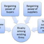
Amazon Porter’s Five Forces Analysis

Porter’s Five Forces analytical framework developed by Michael Porter (1979)[1] represents five individual forces that shape the overall extent of competition in the industry. The essence of Amazon Porter’s Five Forces is represented in figure below:   Threat of new … Continue reading →

The post Amazon Porter’s Five Forces Analysis appeared first on Research-Methodology.

Graph question for growth model "xtmixed"

Hi, I'm having a problem in making a line graph for my growth model.
The outcome variable is depression level: dep_ (categorical)
The main independent variable is gender: sex_ (coded as 0/1)
One time-varying variable is alcohol use: alcohol_new (coded as 0/1)
Time variable is: year_new (4 waves coded as 0, 1, 2 3)
My original command is: xtmixed dep_ sex_ alcohol_new year_new i.sex_#c.year_new i.alcohol_new#c.year_new|| id: year , cov(un) variance mle
I'm wondering how could I do the predict function and then make a line graph which fits this model the best.
Thank you!

Seemingly Unrelated Regression with endogeneity and sample selection

Hello everyone!
I wish to see the impact of income from an activity on various types of household expenditure. Thus, i wish to use seemingly-unrelated regression. However, i am facing two issues here. First, not all the individuals are involved in that activity leading to the problem of sample selection. Also, there is a potential simultaneity between income from that activity and household expenditure leading to the problem of endogeneity.
Can anyone help me with which model to use in a such a situation? Or is there any manual two-step procedure for this?
Thanks

Reassigning records with missing values to existing categories considering the existing distribution within the population

Dear Statalist,

I am struggling to reassign records with a missing value on the categorical variable that assigns each record to a province. I would like to semi-randomly reassign those with a missing value to existing provinces based on the existing frequency within each province. Below I created an example where I had 20 records already assigned to each province, I am also reporting overall frequency for each province. I would like to reassign semi-randomly the three missing values considering the existing frequency for each province. I am using Stata 14 MP.

Thanks



clear
input float(province sex freq)
1 1 .15
1 1 .15
1 2 .15
2 1 .1
2 2 .1
3 2 .1
3 2 .1
4 2 .25
4 2 .25
4 1 .25
4 1 .25
4 1 .25
5 2 .1
5 1 .1
6 2 .1
6 1 .1
7 1 .05
8 1 .05
9 2 .1
9 2 .1
. 2 .
. 1 .
. 1 .
end

Removing duplicates across several variables in panel data and keep the dup with non-missing values

Hi

As the title suggests, I am trying to remove duplicate values across several variables (c30) in a panel data set (sorted by firm id and year), so for example for Firm 3 there are two 2012 rows and one has observations for the variables and one has missing values.

I have looked in a couple of other similar posts and in Nick Cox's notes on the topic in general but I have been unable to come up with a solution.

The code I have tried is:

Code:

collapse (firstnm) `vbles', by(BvDIDnumber Year)

This gave me an error message saying 'varlist required'.

If I enter the names of all variables instead of 'vbles' the error persists.

Apologies if I have missed something in the notes I mentioned, which are always extremely useful for various things I've done I'd liek to add.

Thanks in advance,
Paul

xtreg

hello,

I have a dataset on which I want to perform an OLS. The dataset looks like this:
dependent variable: percentage change of carbon emission of each firm between 2013 and 2018
dependent variables: mean of various firm characteristics from 2010 to 2012.

However, note that I started from a panel dataset to construct this sample, but in my final sample i have only one observation per firm per variable. Am I still able to perform xtreg? Because whenever I try to do this, all my variables are omitted automatically.

Kind regards,
Timea De Wispelaere

Problem with saving graphs with wildcard in names

Hi there!

I'm having some difficulties saving and combining graphs that I have created using a foreach loop and the mrgraph command. The problem seems to be related to the fact that I'm using a wildcard with the mrtab command, but the resulting graphs can't be saved with the "*" in their name (because I suppose it is invalid syntax).

I'm using the following code:

local Q1a1vars Q1a1_*
local Q1a2vars Q1a2_*
local mrvars `Q1a1vars' `Q1a2vars'

foreach var of local mrvars {
mrtab `var'
mrgraph hbar `var' , stat(col) name(`var')
}

where the local Q1a1vars, for example, contains Q1a1_a Q1a1_b Q1a1_c etc. (which is why I use the wildcard). mrvars is therefore a local of locals. In the actual dataset, I hope to perform this foreach loop over a total of 33 similarly constructed locals, but I'm just including two here so as to not over-complicate things.

I'm able to successfully generate the graphs using mrgraph, it's just the naming that is a problem.

Does anyone have any advice about how I could name the graphs?

Please let me know if any additional information is needed!
-Alec

Writing GMM moment conditions for IPW

Hi all,

I am trying to estimate the ATE of an IPW model by writing a GMM code. I am having trouble writing the moment conditions.

gmm (eq1: treatment - invlogit({xb: $xt _cons})) (eq2: (treatment - invlogit({xb: $xt _cons})/((invlogit({xb: $xt _cons})*(1 - invlogit({xb: $xt _cons})))))-{ate}), instruments($xt) onestep

But stata doesn't like them.

Could someone point me in the right direction?

Thanks

Stata evalautes what comes after an if statement that it's not true

Hi all,

I have a do-file (Testing ceqef.do, attached) which I'm using to test an ado-file (ceqef.ado, attached). For the sake of simplicity, I copy the relevant part of the ado-file:

Code:

                    if (wordcount("`tax_`rw'_`cc''")>0 | wordcount("`ben_`rw'_`cc''")>0){ ;  //  #1
                            *impact effectiveness;
                            /*if wordcount("`benef'")>0{;
                                ceqbenstar [w=`w'], endinc(``cc'') ben(`benef');
                            };
                            if wordcount("`taxesef'")>0{;
                                ceqtaxstar [w=`w'], endinc(``cc'') taxes(`taxesef');
                            };*/
                            if (wordcount("`tax_`rw'_`cc''")>0 & wordcount("`ben_`rw'_`cc''")>0) {; //  #2
                                tempvar ystar;
                                gen double `ystar'=``rw'';
                                *set trace on ;
                                ceqtaxstar `pw', startinc(``rw'') taxes(`taxesef');    
                                *set trace off ;
                                local twarn = 0 ; 
                                if r(t_gr) == 1{ ;
                                    nois `dit'  "Sum of `tname_`rw'_`cc'' exceed ``rw'', so impact effectiveness indicator not produced from ``rw'' to ``cc''" ;
                                    local warning `warning'  "Sum of `tname_`rw'_`cc'' exceed ``rw'', so impact effectiveness indicator not produced from ``rw'' to ``cc''" ;
                                    local twarn = r(t_gr) ; 
                                } ;
                                else if r(t_0) == 1{ ;
                                    nois `dit'  "Sum of `tname_`rw'_`cc'' is 0, so impact effectiveness indicator not produced from ``rw'' to ``cc''" ;
                                    local warning `warning'  "Sum of `tname_`rw'_`cc'' exceed ``rw'', so impact effectiveness indicator not produced from ``rw'' to ``cc''" ;
                                    local twarn = r(t_0) ; 
                                } ;
                            
                                ceqbenstar `pw', startinc(``rw'') ben(`benef');
                                local bwarn = 0 ;
                                if r(b_gr) ==1 { ;
                                    nois `dit' "Sum of `bname_`rw'_`cc'' exceed ``rw'', so impact effectiveness indicator for ``rw'' to ``cc'' excludes benefits or is not produced" ;
                                    local warning `warning' "Sum of `bname_`rw'_`cc'' exceed ``rw'', so impact effectiveness indicator for ``rw'' to ``cc'' excludes benefits or is not produced" ;
                                    local bwarn = r(b_gr) ;
                                } ;
                                else if r(b_0) ==1 { ;
                                    nois `dit' "Sum of `bname_`rw'_`cc'' exceed ``rw'', so impact effectiveness indicator for ``rw'' to ``cc'' excludes benefits or is not produced" ;
                                    local warning `warning' "Sum of `bname_`rw'_`cc'' exceed ``rw'', so impact effectiveness indicator for ``rw'' to ``cc'' excludes benefits or is not produced" ;
                                    local bwarn = r(b_0) ;
                                } ;
                                
                                if `bwarn' == 0 & `twarn' == 0 { ;
                                    replace `ystar'=____ybenstar if ____id_benstar==1 & ____id_taxstar!=1;
                                    replace `ystar'=____ytaxstar if ____id_taxstar==1 & ____id_benstar!=1;
                                    tempvar temptax;
                                    gen double    `temptax'=``rw''-    ____ytaxstar if ____id_benstar==1 & ____id_taxstar==1;            
                                    tempvar tempben;
                                    gen double    `tempben'=    ____ybenstar - ``rw'' if ____id_benstar==1 & ____id_taxstar==1;
                                    replace `ystar'=``rw'' - `temptax' +`tempben' if ____id_benstar==1 & ____id_taxstar==1;            
                                    cap drop ____ytaxstar ____ybenstar ____id_benstar ____id_taxstar ;
                                    cap drop `temptax' `tempben';
                                };
                                else  { ;
                                    local bwarn = 1 ;
                                    local twarn = 1 ;
                                };
                            };
                            if (wordcount("`tax_`rw'_`cc''")>0 & wordcount("`ben_`rw'_`cc''")==0) {;  // #3
                                *set trace on;
                                ceqtaxstar `pw' , startinc(``rw'') taxes(`taxesef') ;
                                *set trace off;
                                local twarn = 0 ;
                                if  r(t_gr) ==1 { ;
                                    nois `dit' "Sum of `tname_`rw'_`cc'' exceed ``rw'', so impact effectiveness indicator not produced from ``rw'' to ``cc''" ;
                                    local warning `warning' "Sum of `tname_`rw'_`cc'' exceed ``rw'', so impact effectiveness indicator not produced from ``rw'' to ``cc''" ;                                
                                    local twarn = r(t_gr) ; 
                                } ;
                                else if  r(t_0) ==1 { ;
                                    nois `dit' "Sum of `tname_`rw'_`cc'' is 0, so impact effectiveness indicator not produced from ``rw'' to ``cc''" ;
                                    local warning `warning' "Sum of `tname_`rw'_`cc'' is 0, so impact effectiveness indicator not produced from ``rw'' to ``cc''" ;                                
                                    local twarn = r(t_0) ; 
                                } ;
                                else !(r(t_0) == 1 | r(t_gr) == 1) {;
                                    tempvar ystar;
                                    gen double `ystar'=____ytaxstar;
                                    cap drop ____ytaxstar ____ybenstar ____id_benstar ____id_taxstar;
                                };
                            };
                            if (wordcount("`tax_`rw'_`cc''")==0 & wordcount("`ben_`rw'_`cc''")>0) {;  // #4
                                ceqbenstar `pw', startinc(``rw'') ben(`benef');        
                                local bwarn = 0 ;
                                if r(b_gr) == 1 { ;
                                    nois `dit' "Sum of `bname_`rw'_`cc'' is 0, so impact effectiveness indicator not produced from ``rw'' to ``cc''" ;
                                    local warning `warning' "Sum of `bname_`rw'_`cc'' exceed ``rw'', so impact effectiveness indicator not produced from ``rw'' to ``cc''" ;
                                    local bwarn = r(b_gr) ;
                                } ;
                                else if r(b_0) == 1 { ;
                                    nois `dit' "Sum of `bname_`rw'_`cc'' is 0, so impact effectiveness indicator not produced from ``rw'' to ``cc''" ;
                                    local warning `warning' "Sum of `bname_`rw'_`cc'' exceed ``rw'', so impact effectiveness indicator not produced from ``rw'' to ``cc''" ;
                                    local bwarn = r(b_0) ;
                                } ;
                                if !(r(b_0) == 1 | r(b_gr) == 1) {;            
                                    tempvar ystar;
                                    gen double `ystar'=____ybenstar;
                                    cap drop ____ytaxstar ____ybenstar ____id_benstar ____id_taxstar;
                                };
                        };
                    
                           
                            if (!( "`bwarn'" == "1" & "`twarn'" == "1" )) { ; // #5
                                covconc ``cc'' `pw'; //gini of column income;
                                local g1_`cc'=r(gini);
                                di "`rw' ``rw''";
                                covconc ``rw'' `pw'; //gini of row income;
                                local g2_`rw'=r(gini);
                                covconc `ystar' `pw'; //gini of star income;
                                local g_star=r(gini);
                                local imef=(`g2_`rw''-`g1_`cc'')/(`g2_`rw''-`g_star');
                                matrix `rw'_ef[1,`_`cc'']=`imef';
                            };

Where I've numbered what I think are the 5 most important -if- statements and the #1 continues after #5 is closed. My problem is that when running the do-file, there are certain cases in which `tax_`rw'_`cc'' and `ben_`rw'_`cc'' don't exist and therefore -if- #1 should be false and I would expect Stata to skip everything inside the brackets corresponding to that -if-. However, even though I've confirmed that, in fact, Stata evaluates -if- #1 as false and skips #2 and #3, it runs -if- #4 and #5 (and since there are variables that are not created when the -if- #1 is false, Stata runs into an error and stops running). You can see this in the relevant part of the log-file that I now copy:

- if (wordcount("`tax_`rw'_`cc''")>0 | wordcount("`ben_`rw'_`cc''")>0){ // #1
= if (wordcount("")>0 | wordcount("")>0){ // #1
if (wordcount("`tax_`rw'_`cc''")>0 & wordcount("`ben_`rw'_`cc''")>0) { // #2
tempvar ystar
gen double `ystar'=``rw''
ceqtaxstar `pw', startinc(``rw'') taxes(`taxesef')
local twarn = 0
if r(t_gr) == 1{
nois `dit' "Sum of `tname_`rw'_`cc'' exceed ``rw'', so impact effectiveness indicator not produced from
> ``rw'' to ``cc''"
local warning `warning' "Sum of `tname_`rw'_`cc'' exceed ``rw'', so impact effectiveness indicator not
> produced from ``rw'' to ``cc''"
local twarn = r(t_gr)
}
else if r(t_0) == 1{
nois `dit' "Sum of `tname_`rw'_`cc'' is 0, so impact effectiveness indicator not produced from ``rw'' t
> o ``cc''"
local warning `warning' "Sum of `tname_`rw'_`cc'' exceed ``rw'', so impact effectiveness indicator not
> produced from ``rw'' to ``cc''"
local twarn = r(t_0)
}
ceqbenstar `pw', startinc(``rw'') ben(`benef')
local bwarn = 0
if r(b_gr) ==1 {
nois `dit' "Sum of `bname_`rw'_`cc'' exceed ``rw'', so impact effectiveness indicator for ``rw'' to ``c
> c'' excludes benefits or is not produced"
local warning `warning' "Sum of `bname_`rw'_`cc'' exceed ``rw'', so impact effectiveness indicator for
> ``rw'' to ``cc'' excludes benefits or is not produced"
local bwarn = r(b_gr)
}
else if r(b_0) ==1 {
nois `dit' "Sum of `bname_`rw'_`cc'' exceed ``rw'', so impact effectiveness indicator for ``rw'' to ``c
> c'' excludes benefits or is not produced"
local warning `warning' "Sum of `bname_`rw'_`cc'' exceed ``rw'', so impact effectiveness indicator for
> ``rw'' to ``cc'' excludes benefits or is not produced"
local bwarn = r(b_0)
}
if `bwarn' == 0 & `twarn' == 0 {
replace `ystar'=____ybenstar if ____id_benstar==1 & ____id_taxstar!=1
replace `ystar'=____ytaxstar if ____id_taxstar==1 & ____id_benstar!=1
tempvar temptax
gen double `temptax'=``rw''- ____ytaxstar if ____id_benstar==1 & ____id_taxstar==1
tempvar tempben
gen double `tempben'= ____ybenstar - ``rw'' if ____id_benstar==1 & ____id_taxstar==1
replace `ystar'=``rw'' - `temptax' +`tempben' if ____id_benstar==1 & ____id_taxstar==1
cap drop ____ytaxstar ____ybenstar ____id_benstar ____id_taxstar
cap drop `temptax' `tempben'
}
else {
local bwarn = 1
local twarn = 1
}
}
if (wordcount("`tax_`rw'_`cc''")>0 & wordcount("`ben_`rw'_`cc''")==0) { // #3
ceqtaxstar `pw' , startinc(``rw'') taxes(`taxesef')
local twarn = 0
if r(t_gr) ==1 {
nois `dit' "Sum of `tname_`rw'_`cc'' exceed ``rw'', so impact effectiveness indicator not produced from
> ``rw'' to ``cc''"
local warning `warning' "Sum of `tname_`rw'_`cc'' exceed ``rw'', so impact effectiveness indicator not
> produced from ``rw'' to ``cc''"
local twarn = r(t_gr)
}
else if r(t_0) ==1 {
nois `dit' "Sum of `tname_`rw'_`cc'' is 0, so impact effectiveness indicator not produced from ``rw'' t
> o ``cc''"
local warning `warning' "Sum of `tname_`rw'_`cc'' is 0, so impact effectiveness indicator not produced
> from ``rw'' to ``cc''"
local twarn = r(t_0)
}
else !(r(t_0) == 1 | r(t_gr) == 1) {
tempvar ystar
gen double `ystar'=____ytaxstar
cap drop ____ytaxstar ____ybenstar ____id_benstar ____id_taxstar
}
}
- if (wordcount("`tax_`rw'_`cc''")==0 & wordcount("`ben_`rw'_`cc''")>0) { // #4
= if (wordcount("")==0 & wordcount("")>0) {
ceqbenstar `pw', startinc(``rw'') ben(`benef')
local bwarn = 0
if r(b_gr) == 1 {
nois `dit' "Sum of `bname_`rw'_`cc'' is 0, so impact effectiveness indicator not produced from ``rw'' t
> o ``cc''"
local warning `warning' "Sum of `bname_`rw'_`cc'' exceed ``rw'', so impact effectiveness indicator not
> produced from ``rw'' to ``cc''"
local bwarn = r(b_gr)
}
else if r(b_0) == 1 {
nois `dit' "Sum of `bname_`rw'_`cc'' is 0, so impact effectiveness indicator not produced from ``rw'' t
> o ``cc''"
local warning `warning' "Sum of `bname_`rw'_`cc'' exceed ``rw'', so impact effectiveness indicator not
> produced from ``rw'' to ``cc''"
local bwarn = r(b_0)
}
if !(r(b_0) == 1 | r(b_gr) == 1) {
tempvar ystar
gen double `ystar'=____ybenstar
cap drop ____ytaxstar ____ybenstar ____id_benstar ____id_taxstar
}
}
- assert !( "`bwarn'" == "1" & "`twarn'" == "1" )
= assert !( "" == "1" & "" == "1" )
- pause: pause2
pause: : pause2
-> . q
execution resumes...
- if (!( "`bwarn'" == "1" & "`twarn'" == "1" )) { // #5
= if (!( "" == "1" & "" == "1" )) {
- covconc ``cc'' `pw'
= covconc OI [pw = __000001]
- local g1_`cc'=r(gini)
= local g1_mp=r(gini)
- di "`rw' ``rw''"
= di "m OI"
- covconc ``rw'' `pw'
= covconc OI [pw = __000001]
- local g2_`rw'=r(gini)
= local g2_m=r(gini)
- covconc `ystar' `pw'
= covconc [pw = __000001]
varlist required
local g_star=r(gini)
local imef=(`g2_`rw''-`g1_`cc'')/(`g2_`rw''-`g_star')
matrix `rw'_ef[1,`_`cc'']=`imef'
}

Since I set the trace on, you can clearly see which -if- statements run. I really don't understand why. I've checked multiple times if all the -if- statements were properly closed, and as far as I can tell, they are. Can you think of another reason why this -if- statement is not working as it should (others in the ado-file work perfectly fine)?

Many thanks in advance for your help!

Never allow Stata to replace dataset

I have ingrained in my muscle memory to press "ctrl+s" every time before I run a .do file in case Stata crashes. Once in a while I write code directly into the Stata command field, especially when I tabulate or summarise variables I just created to quality check them. I have thus accidently managed to press "ctrl+s" while in this window accidentaly, and followingly press enter with the intent to execute the command I wrote into the command window. This of course, replaces the data set I am working on, which I extremely seldomly want to do, and especially not outside of a .do file.

Is there a way to never allow Stata to overwrite a specific file? In the .do file I use the "replace" option to force Stata to overwrite, but I could not find any options to "lock" the data set. I couldn't find an option anywhere to dissalow the "ctrl+s" on saving data sets. I wanted to ask if there is some information I am missing?

Merging data

Hello,

I am trying to merge variables from the original Demographic and Health surveys (DHS) with the IPUMS-DHS data. The unique identifier in both datasets is "caseid". My master dataset (IPUMS) has a caseid and year variable (2005 and 2014) plus all other measures. In the original DHS they also have caseid, year variable (2005 ONLY) plus another variable which I would like to merge in.



I run the following command using my master dataset:

Code:

merge m:1 caseid year using "original DHS data file"

Which returns the following:

Code:

    Result                           # of obs.
    -----------------------------------------
    not matched                       126,364
        from master                   106,890  (_merge==1)
        from using                     19,474  (_merge==2)

    matched                                 0  (_merge==3)
    -----------------------------------------

Nothing has been matched. I have tried m:1 and 1:1 and I get the same result. Can anyone advise?

Blinder-Oaxaca decomposition for probit model

Hello,

I have assessed online materials available for the decomposition of both linear and non-linear models but am not quite understanding the correct code to use in the current context.

I have obtained results for the average predicted probabilities (of being employed (emp = 1 if employed, 0= otherwise)) of non-disabled (DISTYPE = 4) and work-limited disabled (DISTYPE =1) via:

Code:

 probit emp DISTYPE SEX ETH AGES1 URESMC1 HDPCH191 IND1 MARSTA1 HIQUAL81 REGWKR1 SKSBN911 FTPTWK1, nolog 

margins, at(DISTYPE=(1 4)) vsquish

I believe the following format is adequate:

Code:

 fairlie depvar indepvars [if] [in] [weight], by(groupvar) [ options ]

But I am struggling how to integrate these results (the average predicted probabilities for both groups) to decompose the differences in observed characteristics and the 'unexplained' gap, for male and female?

Any help would be greatly appreciated.

Replacing missing values in a panel data

Dear All,

hope you are all safe and in good health.

Kindly I have balanced panel data with missing values for some years, I am interested in two specific years, where I want to replace years (e.i. 2000 and 2015) with values from previous or onwards years, in particular:
1- I want to replace the year 2000 (if no value) with a value from the closest onward years till 2006 e.g. 2001, (if no value available in 2001), then from 2002, (if no value, then till ... 2006), the year 2000 will have no value in case years 2001 to 2006 don't have any values.

2- For the year 2015, I want to replace (if no value) with a value from the closest years, first by going backward from 2014 to 2010, in case of no values for years 2014 to 2016, then I want to replace 2015 (if no value), by going onward from 2016 till 2018, the year 2015 will have no value in case the years 2010 till the latest year don't have any value.

- The dataset has 22 countries for 167 indicators (seriescode) spanning the period 2000 to 2019, kindly find below an example of the dataset

- The variable id is the combination of (goal target indicator seriescode concatenate) using group command in egen.

- dum_year is a dummy variable denoting 1 if year <2007, 2 if year between 2010 and 2015, 3 if year 2016 and above.

- Years 2007 to 2009 are dropped.

I tried the following code to fill/ replace the year 2000, but it didn't work:

Code:

bys geoarename id: replace value=value[_n+1] if value==. & dum+_year==1

Any help and advice on how to fill the years 2000 and 2015.

Thank you so much.

stay safe,

Rabih

----------------------- copy starting from the next line -----------------------

Code:

* Example generated by -dataex-. To install: ssc install dataex
clear
input byte goal float dum_year str5 target str7 indicator str17 seriescode str20 geoareaname float(timeperiod value id) str42 concatenate
1 1 "1.1" "1.1.1" "SI_POV_DAY1" "Djibouti"           2000    .  1 ";;;;;;;;;;;;;;;;;G;"          
1 1 "1.1" "1.1.1" "SI_POV_DAY1" "Djibouti"           2001    .  1 ";;;;;;;;;;;;;;;;;G;"          
1 1 "1.1" "1.1.1" "SI_POV_DAY1" "Djibouti"           2002 20.6  1 ";;;;;;;;;;;;;;;;;G;"          
1 1 "1.1" "1.1.1" "SI_POV_DAY1" "Djibouti"           2003    .  1 ";;;;;;;;;;;;;;;;;G;"          
1 1 "1.1" "1.1.1" "SI_POV_DAY1" "Djibouti"           2004    .  1 ";;;;;;;;;;;;;;;;;G;"          
1 1 "1.1" "1.1.1" "SI_POV_DAY1" "Djibouti"           2005    .  1 ";;;;;;;;;;;;;;;;;G;"          
1 1 "1.1" "1.1.1" "SI_POV_DAY1" "Djibouti"           2006    .  1 ";;;;;;;;;;;;;;;;;G;"          
1 2 "1.1" "1.1.1" "SI_POV_DAY1" "Djibouti"           2010    .  1 ";;;;;;;;;;;;;;;;;G;"          
1 2 "1.1" "1.1.1" "SI_POV_DAY1" "Djibouti"           2011    .  1 ";;;;;;;;;;;;;;;;;G;"          
1 2 "1.1" "1.1.1" "SI_POV_DAY1" "Djibouti"           2012 18.3  1 ";;;;;;;;;;;;;;;;;G;"          
1 2 "1.1" "1.1.1" "SI_POV_DAY1" "Djibouti"           2013 22.7  1 ";;;;;;;;;;;;;;;;;G;"          
1 2 "1.1" "1.1.1" "SI_POV_DAY1" "Djibouti"           2014    .  1 ";;;;;;;;;;;;;;;;;G;"          
1 2 "1.1" "1.1.1" "SI_POV_DAY1" "Djibouti"           2015    .  1 ";;;;;;;;;;;;;;;;;G;"          
1 3 "1.1" "1.1.1" "SI_POV_DAY1" "Djibouti"           2016    .  1 ";;;;;;;;;;;;;;;;;G;"          
1 3 "1.1" "1.1.1" "SI_POV_DAY1" "Djibouti"           2017 17.1  1 ";;;;;;;;;;;;;;;;;G;"          
1 3 "1.1" "1.1.1" "SI_POV_DAY1" "Djibouti"           2018    .  1 ";;;;;;;;;;;;;;;;;G;"          
1 3 "1.1" "1.1.1" "SI_POV_DAY1" "Djibouti"           2019    .  1 ";;;;;;;;;;;;;;;;;G;"          
1 1 "1.1" "1.1.1" "SI_POV_DAY1" "State of Palestine" 2000    .  1 ";;;;;;;;;;;;;;;;;G;"          
1 1 "1.1" "1.1.1" "SI_POV_DAY1" "State of Palestine" 2001    .  1 ";;;;;;;;;;;;;;;;;G;"          
1 1 "1.1" "1.1.1" "SI_POV_DAY1" "State of Palestine" 2002    .  1 ";;;;;;;;;;;;;;;;;G;"          
1 1 "1.1" "1.1.1" "SI_POV_DAY1" "State of Palestine" 2003    .  1 ";;;;;;;;;;;;;;;;;G;"          
1 1 "1.1" "1.1.1" "SI_POV_DAY1" "State of Palestine" 2004  1.1  1 ";;;;;;;;;;;;;;;;;G;"          
1 1 "1.1" "1.1.1" "SI_POV_DAY1" "State of Palestine" 2005   .9  1 ";;;;;;;;;;;;;;;;;G;"          
1 1 "1.1" "1.1.1" "SI_POV_DAY1" "State of Palestine" 2006   .3  1 ";;;;;;;;;;;;;;;;;G;"          
1 2 "1.1" "1.1.1" "SI_POV_DAY1" "State of Palestine" 2010   .2  1 ";;;;;;;;;;;;;;;;;G;"          
1 2 "1.1" "1.1.1" "SI_POV_DAY1" "State of Palestine" 2011   .2  1 ";;;;;;;;;;;;;;;;;G;"          
1 2 "1.1" "1.1.1" "SI_POV_DAY1" "State of Palestine" 2012    .  1 ";;;;;;;;;;;;;;;;;G;"          
1 2 "1.1" "1.1.1" "SI_POV_DAY1" "State of Palestine" 2013    .  1 ";;;;;;;;;;;;;;;;;G;"          
1 2 "1.1" "1.1.1" "SI_POV_DAY1" "State of Palestine" 2014    .  1 ";;;;;;;;;;;;;;;;;G;"          
1 2 "1.1" "1.1.1" "SI_POV_DAY1" "State of Palestine" 2015    .  1 ";;;;;;;;;;;;;;;;;G;"          
1 3 "1.1" "1.1.1" "SI_POV_DAY1" "State of Palestine" 2016    1  1 ";;;;;;;;;;;;;;;;;G;"          
1 3 "1.1" "1.1.1" "SI_POV_DAY1" "State of Palestine" 2017    .  1 ";;;;;;;;;;;;;;;;;G;"          
1 3 "1.1" "1.1.1" "SI_POV_DAY1" "State of Palestine" 2018    .  1 ";;;;;;;;;;;;;;;;;G;"          
1 3 "1.1" "1.1.1" "SI_POV_DAY1" "State of Palestine" 2019    .  1 ";;;;;;;;;;;;;;;;;G;"          
1 1 "1.1" "1.1.1" "SI_POV_EMP1" "State of Palestine" 2006   .1  2 "15+;BOTHSEX;;;;;;;;;;;;;;;;G;"
1 1 "1.1" "1.1.1" "SI_POV_EMP1" "State of Palestine" 2005   .2  2 "15+;BOTHSEX;;;;;;;;;;;;;;;;G;"
1 1 "1.1" "1.1.1" "SI_POV_EMP1" "State of Palestine" 2004   .3  2 "15+;BOTHSEX;;;;;;;;;;;;;;;;G;"
1 1 "1.1" "1.1.1" "SI_POV_EMP1" "State of Palestine" 2003    .  2 "15+;BOTHSEX;;;;;;;;;;;;;;;;G;"
1 1 "1.1" "1.1.1" "SI_POV_EMP1" "State of Palestine" 2002    .  2 "15+;BOTHSEX;;;;;;;;;;;;;;;;G;"
1 1 "1.1" "1.1.1" "SI_POV_EMP1" "State of Palestine" 2001    .  2 "15+;BOTHSEX;;;;;;;;;;;;;;;;G;"
1 1 "1.1" "1.1.1" "SI_POV_EMP1" "State of Palestine" 2000    .  2 "15+;BOTHSEX;;;;;;;;;;;;;;;;G;"
1 2 "1.1" "1.1.1" "SI_POV_EMP1" "State of Palestine" 2015    .  2 "15+;BOTHSEX;;;;;;;;;;;;;;;;G;"
1 2 "1.1" "1.1.1" "SI_POV_EMP1" "State of Palestine" 2014    .  2 "15+;BOTHSEX;;;;;;;;;;;;;;;;G;"
1 2 "1.1" "1.1.1" "SI_POV_EMP1" "State of Palestine" 2013    .  2 "15+;BOTHSEX;;;;;;;;;;;;;;;;G;"
1 2 "1.1" "1.1.1" "SI_POV_EMP1" "State of Palestine" 2012    .  2 "15+;BOTHSEX;;;;;;;;;;;;;;;;G;"
1 2 "1.1" "1.1.1" "SI_POV_EMP1" "State of Palestine" 2011   .1  2 "15+;BOTHSEX;;;;;;;;;;;;;;;;G;"
1 2 "1.1" "1.1.1" "SI_POV_EMP1" "State of Palestine" 2010    0  2 "15+;BOTHSEX;;;;;;;;;;;;;;;;G;"
1 3 "1.1" "1.1.1" "SI_POV_EMP1" "State of Palestine" 2019    .  2 "15+;BOTHSEX;;;;;;;;;;;;;;;;G;"
1 3 "1.1" "1.1.1" "SI_POV_EMP1" "State of Palestine" 2018    .  2 "15+;BOTHSEX;;;;;;;;;;;;;;;;G;"
1 3 "1.1" "1.1.1" "SI_POV_EMP1" "State of Palestine" 2017   .2  2 "15+;BOTHSEX;;;;;;;;;;;;;;;;G;"
1 3 "1.1" "1.1.1" "SI_POV_EMP1" "State of Palestine" 2016    .  2 "15+;BOTHSEX;;;;;;;;;;;;;;;;G;"
1 1 "1.1" "1.1.1" "SI_POV_EMP1" "Jordan"             2006   .3 10 "25+;MALE;;;;;;;;;;;;;;;;G;"   
1 1 "1.1" "1.1.1" "SI_POV_EMP1" "Jordan"             2005    . 10 "25+;MALE;;;;;;;;;;;;;;;;G;"   
1 1 "1.1" "1.1.1" "SI_POV_EMP1" "Jordan"             2004    . 10 "25+;MALE;;;;;;;;;;;;;;;;G;"   
1 1 "1.1" "1.1.1" "SI_POV_EMP1" "Jordan"             2003   .9 10 "25+;MALE;;;;;;;;;;;;;;;;G;"   
1 1 "1.1" "1.1.1" "SI_POV_EMP1" "Jordan"             2002    . 10 "25+;MALE;;;;;;;;;;;;;;;;G;"   
1 1 "1.1" "1.1.1" "SI_POV_EMP1" "Jordan"             2001    . 10 "25+;MALE;;;;;;;;;;;;;;;;G;"   
1 1 "1.1" "1.1.1" "SI_POV_EMP1" "Jordan"             2000    . 10 "25+;MALE;;;;;;;;;;;;;;;;G;"   
1 2 "1.1" "1.1.1" "SI_POV_EMP1" "Jordan"             2015    . 10 "25+;MALE;;;;;;;;;;;;;;;;G;"   
1 2 "1.1" "1.1.1" "SI_POV_EMP1" "Jordan"             2014    . 10 "25+;MALE;;;;;;;;;;;;;;;;G;"   
1 2 "1.1" "1.1.1" "SI_POV_EMP1" "Jordan"             2013    . 10 "25+;MALE;;;;;;;;;;;;;;;;G;"   
1 2 "1.1" "1.1.1" "SI_POV_EMP1" "Jordan"             2012    . 10 "25+;MALE;;;;;;;;;;;;;;;;G;"   
1 2 "1.1" "1.1.1" "SI_POV_EMP1" "Jordan"             2011    . 10 "25+;MALE;;;;;;;;;;;;;;;;G;"   
1 2 "1.1" "1.1.1" "SI_POV_EMP1" "Jordan"             2010   .2 10 "25+;MALE;;;;;;;;;;;;;;;;G;"   
1 3 "1.1" "1.1.1" "SI_POV_EMP1" "Jordan"             2019    . 10 "25+;MALE;;;;;;;;;;;;;;;;G;"   
1 3 "1.1" "1.1.1" "SI_POV_EMP1" "Jordan"             2018    . 10 "25+;MALE;;;;;;;;;;;;;;;;G;"   
1 3 "1.1" "1.1.1" "SI_POV_EMP1" "Jordan"             2017    . 10 "25+;MALE;;;;;;;;;;;;;;;;G;"   
1 3 "1.1" "1.1.1" "SI_POV_EMP1" "Jordan"             2016    . 10 "25+;MALE;;;;;;;;;;;;;;;;G;"   
end

------------------ copy up to and including the previous line ------------------

Spell-type data for Cox regression

Hello, dear users of the Stata program. Now I'm conducting a reserach on duration of unemployment. I want to use Cox regression to determine the probability of exiting unemployment.
I prepared the file with unemployment spells in accordance with Stata journal article https://www.stata-journal.com/sjpdf....iclenum=dm0029.
I obtained 180 spells the defined the beginning and ending months for them, duration and censoring flag.

Do I need to reduce observations within 1 spell just to get number of observations as number of spells?
Because now I have data for each observation from each spell and I can't merge other data set with individual characteristics (gender, age, etc). I think this would be sensible.

if yes, how should I do this? I could not find such instructions and I can't continue the work.

drop all zero variables

Hello,

I have created dummy variables for industries, resulting in 35 dummies. However, I deleteted some observations, resulting in a couple of all zero dummies. I am wondering how to delete these variables most efficiently.

Kind regards,
Timea De Wispelaere

Predictions with and without BLUP after melogit

I am attempting to calculate predictions after a melogit model with and without best linear unbiased predictors. In SAS I would do this as follows:

Code:

PROC GLIMMIX DATA=&ANALYSIS NOCLPRINT MAXLMMUPDATE=100;
CLASS PROVID;
ODS OUTPUT PARAMETERESTIMATES=&EST (KEEP=EFFECT ESTIMATE STDERR);
MODEL OUTCOME=&MODEL_VAR
        /D=B LINK=LOGIT SOLUTION;
XBETA=_XBETA_;
LINP=_LINP_;
RANDOM INTERCEPT/SUBJECT=PROVID SOLUTION;
OUTPUT OUT=OUTCOME
        PRED(BLUP ILINK)=PREDPROB PRED(NOBLUP ILINK)=EXPPROB;

For SAS the options above are:
BLUP=linear predictor
NOBLUP = marginal linear predictor
ILINK = predicted mean

However, in Stata I am not totally sure how to do this. Here is the code I am using. My understanding is that the predict command after running an melogit predicts the BLUP at the means. But I am not sure if the xb option would be calculating predictions at the means without the BLUP.

Code:

melogit outcome modelvars  || secondlevel:
predict predicted
predict expected, xb

Three-level mix-effect model for ordered logistic regression in Stata- meologit regression

Dear all,

I am currently working with a cluster data collected from 3229 respondents in 40 counties, half of which are policy pilot sites. The dependent variable is categorical data from 1-5 regarding individuals' attitudes.

I am trying to fit a 3 level mixed-effect model by using the demand of meologit in Stata 15.

The first level: SES + explanatory variable about individuals
The second level: 40 country id
The third level: pilot (0 or 1)
code: meologit urbani A1b A0 marriage i.educat4 occu_prof hhwealth hukou_cat32 hukou_cat33 hukou_out_town_impute1 [pw=weight_temp_use] || pilot1t: || gbcode: , nolog

I am thinking the 3229 individuals are nested with country, and then the 40 counties nest with the pilot, but not sure for the following questions:

1. Is the binary variable (pilot) can be used as the third level control? Especially when considering the group size issue.
(now the third level data is divided into two groups: 20 pilot country and 20 non-pilot country)
2. The results as following show that the variance of pilot is quite large, and what can we tell?
3. Also, there did not show the test result in front of the table...how should I modify my model or code accordingly?

Thank you for your reply if you are familiar with this model.

I really appreciated your help.


Array

Correlation Pb

Hello,

I am pretty new to Stata and econometrics in general so please excuse me if my question seems stupid or is redundant. I really can't manage to find a solution.

I'm working with panel datas (2011 to 2017), on the effect of oil prices on the economic growth with the following pooled OLS regression:
reg growth gvt_spendings fixed_capital_form oil_import_price elec_oil opep beneOpep

The problem is I identified a high correlation between government spendings and the fixed capital formation:

correlate DC_A FBCF
(obs=1,197)

| DC_A FBCF
---------------+------------------------
DC_A | 1.0000
FBCF | 0.8946 1.0000


That could explain the negative effect of government_spendings on growth (which has to be a positive coefficient following GDP=C+I+G):
. reg $ylist $xlist

Source | SS df MS Number of obs = 94
-------------+---------------------------------- F(7, 86) = 6.36
Model | 404.779791 7 57.8256844 Prob > F = 0.0000
Residual | 782.304497 86 9.09656392 R-squared = 0.3410
-------------+---------------------------------- Adj R-squared = 0.2873
Total | 1187.08429 93 12.7643472 Root MSE = 3.0161

------------------------------------------------------------------------------
croissance | Coef. Std. Err. t P>|t| [95% Conf. Interval]
-------------+----------------------------------------------------------------
gvt | -1.90e-11 4.70e-12 -4.04 0.000 -2.83e-11 -9.64e-12
FCF | 2.31e-11 5.20e-12 4.44 0.000 1.27e-11 3.34e-11
Kb_ent | -1.41e-12 3.54e-13 -3.98 0.000 -2.11e-12 -7.05e-13
pOILimport | -.0388874 .0143319 -2.71 0.008 -.0673783 -.0103965
ÉLECoil | -.476328 .1116277 -4.27 0.000 -.6982365 -.2544195
OPEP | -.0234799 .814232 -0.03 0.977 -1.64212 1.59516
béné_OPEP | -.0904356 .14431 -0.63 0.533 -.3773145 .1964432
_cons | 6.269373 1.486281 4.22 0.000 3.314744 9.224002
--------------------------------------------------------------------------



The only way I found to solve my correlation problem could be to drop government_spendings, but p-values skyrocket and my R^2 decreases a lot:

. reg $ylist $xlist

Source | SS df MS Number of obs = 94
-------------+---------------------------------- F(6, 87) = 3.40
Model | 225.735623 6 37.6226038 Prob > F = 0.0046
Residual | 961.348665 87 11.0499847 R-squared = 0.1902
-------------+---------------------------------- Adj R-squared = 0.1343
Total | 1187.08429 93 12.7643472 Root MSE = 3.3242

------------------------------------------------------------------------------
croissance | Coef. Std. Err. t P>|t| [95% Conf. Interval]
-------------+----------------------------------------------------------------
gvt | 4.61e-13 1.87e-12 0.25 0.806 -3.26e-12 4.18e-12
Kb_ent | -9.48e-14 2.13e-13 -0.44 0.658 -5.19e-13 3.29e-13
pOILimport | -.0367706 .0157872 -2.33 0.022 -.0681494 -.0053918
ÉLECoil | -.4131606 .122026 -3.39 0.001 -.6557004 -.1706208
OPEP | .7600824 .8760425 0.87 0.388 -.9811469 2.501312
béné_OPEP | -.0518004 .158762 -0.33 0.745 -.367357 .2637562
_cons | 6.083269 1.637458 3.72 0.000 2.828645 9.337894
-----------------------------------------------------------------------------


Is there a way to solve this problem of correlation? or making those p-values significant?
Keep FCF in the regression would be nice too.



Thanks a lot

Composite Index

Hi! I am trying to generate a composite index for 2 numerical variables. what is the best way to do it? This question may sound stupid but I am really stuck here.
Thanks in advance!

Sample size & power for quantile regression

Hello,

For a clinical trial using quantile regression to test the null hypothesis, could anyone advise on the correct method to use to determine the sample size/power?

Thanks for your help,
Megan

DID (Differences-in-difference) regression

Dear All, I’m having a problem with DID regression equation. I am using Stata 12.

when I ran the regression

xtreg lnDSL DID ADD EDD SRD BD Inflation LFTA PUCTA TDTA lnTA INVSTA,r

Random-effects GLS regression Number of obs = 4728
Group variable: i Number of groups = 72

R-sq: within = 0.8080 Obs per group: min = 58
between = 0.9538 avg = 65.7
overall = 0.9332 max = 66

Wald chi2(11) = 3116.91
corr(u_i, X) = 0 (assumed) Prob > chi2 = 0.0000

(Std. Err. adjusted for 72 clusters in i)

Robust
lnDSL Coef. Std. Err. z P>z [95% Conf. Interval]

DID .0083772 .0605678 0.14 0.890 -.1103334 .1270878
ADD .168977 .0391338 4.32 0.000 .0922762 .2456778
EDD -.1419524 .0356399 -3.98 0.000 -.2118054 -.0720995
SRD -.0885526 .1545537 -0.57 0.567 -.3914723 .2143671
BD -.4985233 .2932512 -1.70 0.089 -1.073285 .0762385
Inflation .0029831 .0032751 0.91 0.362 -.0034359 .0094021
LFTA -.0068422 .0039584 -1.73 0.084 -.0146005 .0009161
PUCTA -.0089974 .0087924 -1.02 0.306 -.0262302 .0082354
TDTA .0112309 .003142 3.57 0.000 .0050727 .0173892
lnTA 1.130584 .0802098 14.10 0.000 .9733753 1.287792
INVSTA -.0101493 .0039944 -2.54 0.011 -.0179781 -.0023205
_cons -5.251152 .7122417 -7.37 0.000 -6.64712 -3.855184

sigma_u .36208126
sigma_e .31319664
rho .57201446 (fraction of variance due to u_i)

I am wondering why DID model is giving me the result of Random-effects GLS regression .


Thank You

Help with merging two datasets

Dear all,

I am using Stata 16, on mac. I have attached the two excel datasets that I am working with for my project. Both have a variable named movie_title. I want to merge two datasets, so that I will end up with one that has the movie_title, rotten_tomatometer_score, and opening weekend revenue. The problem is that the movies in each of the datasets are not entirely the same and are not in the same order. For example, the first dataset will have Deadpool in the first column but the other has Deadpool in column 50. There are also movies in the second dataset that are not in the first one. For example, the first will have the movie Star Trek Beyond, but the other will not. Does anyone have an idea how I can merge these two together? I honestly have no idea on what to do and would greatly appreciate any help on how to solve this!

Thank you in advance for your help

Jason Browen

replace with the last row in each goup

Hi STATALIST,

Could you please help me to replace meacstdivol_1 with last row within each study_1?

Code:

study_1	meanctdivol_1
8363
8363
8363	12.6
8363
8363
8363	12.3
8363
8363
8363	12.5
8363	12.4
10642
10642
10642	45.8
10642	45.8

so results should be like:

Code:

study_1	meanctdivol_1	ctdi
8363		12.4
8363		12.4
8363	12.6	12.4
8363		12.4
8363		12.4
8363	12.3	12.4
8363		12.4
8363		12.4
8363	12.5	12.4
8363	12.4	12.4
10642		45.8
10642		45.8
10642	45.8	45.8
10642	45.8	45.8

Kind regards,

Problem with variables names inside loops

Hi all,

I have a set of variables named "ratio_##########_co_###" (where # are numbers).

My problem is when applying loops as:

Code:

 summarize ratio_`k'_co_`j'

The problem is that summarize interprets, for example:

Code:

summarize ratio_0101100010_co_3

Which does not exist in my dataset, as if it were:

Code:

summarize ratio_0101100010_co_38

Which exists in my dataset.
So the summarize is bringing me the same values for both variables despite "ratio_0101100010_co_3" does not exist.
It is like the system is interpreting the variable having the end 3 as the first digit and analyzing an existing variable with other digits but beginning with the 3.

Hope I am clear enough.
Thanks!

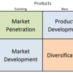
Amazon Ansoff Matrix

Amazon Ansoff Matrix is a marketing planning model that helps the e-commerce and cloud computing company to determine its product and market strategy. Ansoff Matrix illustrates four different strategy options available for businesses.  These are market penetration, product development, market … Continue reading →

The post Amazon Ansoff Matrix appeared first on Research-Methodology.

Fine and Gray calculate individual risks

Dear all,

I would like to calculate the 10-year risk of stroke for each individual in my dataset, given a set of baseline covariates.
I am having troubles estimating 10-year individual risks based on a Fine and Gray model.
For a Cox model, I calculate 10-year risk using the following commands:

stset studytime, failure(stroke=1)
stcox age BP sm
predict double xb, xb
predict double basesurv, basesurv
sum basesurv if _t<10
scalar base10y=r(min)
gen risk10y=1 - base10y^exp(xb)
replace risk10y=risk10y*100


Now the question is, is it possible to calculate the 10-year risks of each individual in my dataset after running a Fine and Gray model?
stcrreg age BP sm, compete(stroke_compete=2)

I would very much appreciate your thoughts.

Best,
John

Dummy variables in first difference regression

Hi guys,

I have a potentially very stupid question to ask, but for the life of me I can not figure this out.

I am estimating cartel damages using a dummy variable approach. Essentially I am setting my "cartel dummy" equal to 1 during the cartel and 0 otherwise, as is the standard approach. However, the other variables in my model are non-stationary and as such I am estimating the regression equation in first differences.

When using a level regression, the interpretation of the dummy is relatively straightforward - one can more or less directly compute the percentage overcharge from the coefficient on the dummy variable. Basically, it shows by what percentage was higher but-for the cartel.

My question is, how would one interpret the coefficient on such a dummy variable when all the regressors in the model are in first differences?

Thanks!
Albertus

line graphic of series from 1st occurrence Covid-19

Hello!
I am using the data set provided in this study, "Oxford COVID-19 govt response tracker' here to graph the different measures implemented by states from the beginning of the Covid-19 outbreak in Europe.

Code:

Contains data
  obs:        10,182                          
 vars:            37                          
------------------------------------------------------------------------------------------------------------------------
              storage   display    value
variable name   type    format     label      variable label
------------------------------------------------------------------------------------------------------------------------
CountryName     str32   %32s                  CountryName
CountryCode     str3    %9s                   CountryCode
Date            long    %10.0g                Date
strDate         str8    %9s                   Date
S1_Schoolclos~g byte    %10.0g                S1_School closing
S1_IsGeneral    byte    %10.0g                S1_IsGeneral
S2_Workplacec~g byte    %10.0g                S2_Workplace closing
S2_IsGeneral    byte    %10.0g                S2_IsGeneral
S3_Cancelpubl~s byte    %10.0g                S3_Cancel public events
S3_IsGeneral    byte    %10.0g                S3_IsGeneral
S4_Closepubli~t byte    %10.0g                S4_Close public transport
S4_IsGeneral    byte    %10.0g                S4_IsGeneral
S5_Publicinfo~s byte    %10.0g                S5_Public information campaigns
S5_IsGeneral    byte    %10.0g                S5_IsGeneral
S6_Restrictio~e byte    %10.0g                S6_Restrictions on internal movement
S6_IsGeneral    byte    %10.0g                S6_IsGeneral
S7_Internatio~s byte    %10.0g                S7_International travel controls
S8_Fiscalmeas~s double  %10.0g                S8_Fiscal measures
S9_Monetaryme~s double  %10.0g                S9_Monetary measures
S10_Emergency~l double  %10.0g                S10_Emergency investment in health care
S11_Investmen~s double  %10.0g                S11_Investment in Vaccines
ConfirmedCases  long    %10.0g                ConfirmedCases
ConfirmedDeaths int     %10.0g                ConfirmedDeaths
StringencyIndex byte    %10.0g                StringencyIndex
tsdate          float   %td                  
ctry            long    %8.0g      ctry       CountryCode

tsdate and ctry are generated by me;

My goal is to graph together, comparative, head-to-head, not time delayed, some selected countries (ITA ESP, FRA, ROU) using as reference:
1) days from the first case reported for one graph
2) cumulative number of confirmed cases for another graph.
I declared the set timeseries by ctry and tsdate and used addplot to overlay the four graphs, using for the X reference the lagged time between first case in each country: France having the first case reported (Jan 24), Italy and Spain 8 days later (Jan 31) and Romania 34 days later (Feb 26).
It worked (see below), however the X labels are misleading (of course I can have them removed) and I don't find it very elegant.
Array

Is there a way to do this more directly and having control over the legend?

Regarding the second graph, using the number of cases as the X reference worked by overriding the panel setting with t(ConfirmedCases), but the graph looks like this:
Array
Any ideea how to use the whole plot area?

Thank you!
Best,
Cristian

Quick question: winsor right only & interaction

Dear members

I have 2 very quick questions.

First: I need to winsorize a variable further ONLY on the right side. I think this is done by including 'highonly' in STATA. However it does not seem to work. To be more clear I need to winsorize a winsorized variable again on the right side only.

The formula I use is as follows: -winsor winsorized_variable, gen(win_var_right) p(0.05) highonly
What am I doing wrong? I get the exact same result with win_var_right as in winsorized_variable.

Second: I need to be dealing with an interaction effect as well. I know that I just have to multiply 2 variables. One of these variables is a winsorized one. Do I just multiply the winsorized one & a non-winsorized variable together? It does make sense however I'm not exactly sure.

similar observations within one variable

Hi,

I would like to spot the observations that are very much alike within one string variable.

Let's say for instance that I have a variable with 4 observations, such as:
var1
observation1: "cat"
obs 2: "caty"
obs 3: "the cat is beautiful"
obs 4: "cat"
I would like to have some distance measure that tells me that observation 1 and 4 are equal, observations 1 and 2 are quite similar, but observations 1 and 3 are very different. Is it possible?

Thanks

chi2 test with probability weights

Dears

I would lke to run a chi2 test but using pw rather than fw.
If i use fw stata of course will not account for the proportion of my real sample giving me wrong p-values.
If I compute the chi2 by dividing for the total weighted and moltiplying for the total observed (i.e. ((401/2322)*85) tot number of real observation) I get a not significant test

Considering that the command [pw=weights] is not allowed with tab var1 var2, chi2, is there an alternative to account for the real size of the sample and thus use the pw?
Below an extraction of the database i am using.

Thanks

Code:

. tab mb_predictable kiwi_club [fw=new_w] if country==2,    chi2


          
 business 
predictabe       No-Club       Club      Total

1                       401            146           547 
2                       253              26           279 
3                       417            104           521 
4                       707            126           833 
5                       110              32           142 


Total      1,888        434      2,322 

Pearson chi2(4) =  48.0612   Pr = 0.000

Code:

* Example generated by -dataex-. To install: ssc install dataex
clear
input byte mb_predictable long club float weights
3 1 26
1 1 26
1 1 26
1 0 95
4 0 16
4 0 26
4 0 16
4 0 26
4 0 26
3 0 16
3 0 16
1 1 26
1 0 26
1 0 16
2 0 16
4 1 16
2 0 16
1 0 95
2 0 16
2 0 16
3 1 26
3 0 26
3 0 95
3 0 16
1 0 16
1 0 95
4 0 16
4 1 26
4 1 16
4 0 16
2 0 26
5 0 26
5 0 26
1 0 16
5 0 16
4 0 26
3 1 26
5 0 16
1 0 26
1 1 26
4 0 16
5 1 16
4 0 26
2 0 16
2 0 26
2 0 95
5 0 26
4 0 16
4 0 16
4 0 26
4 0 26
4 0 16
4 0 16
4 1 26
4 0 16
3 1 26
2 1 26
4 0 26
4 0 16
4 1 16
3 0 95
4 0 16
3 0 16
3 0 95
3 0 26
4 0 16
4 0 16
2 0 26
4 1 26
4 0 26
1 1 26
4 0 16
4 0 16
4 0 16
4 0 16
4 0 16
1 0 16
4 0 16
4 0 26
3 0 16
4 0 95
4 0 16
5 1 16
4 0 16
1 1 16
end
label values kiwi_club club
label def club 0 "No-Club", modify
label def club 1 "Club", modify

If statement within foreach

Hey!
So I would like to run a regression if income is within the range of (0-10727.88).

Code:

    local vars "spending inp out"
    foreach var of local vars {
    if `fam_income' <= 10727.88 {
 
eststo:  quietly regress any_`var' rand_plan_group2 rand_plan_group3 rand_plan_group4 rand_plan_group5 rand_plan_group6 demeaned_fam_start_month_site* demeaned_cal_year*, cluster(ifamily)

}

So far I have tried the code above but I get the following error:

Code:

<=10727.88 invalid name
r(198);

Is there another way to do the code or am I missing something? I'm not that familiar with Stata.

Thanks!

Panel data format

Hi
I would like to transform my panel data so that the years are grouped from 1989 to 2016, consecutively, with each of my country observations. This is the type of format that I would like to obtain:

Code:

[ATTACH=CONFIG]temp_17487_1585561202688_248[/ATTACH]

And this is my current data format:

Code:

* Example generated by -dataex-. To install: ssc install dataex
clear
input str48 Time str6 TimeCode str24 CountryName str17 BroadmoneyofGDPFMLBLB
"2016" "YR2016" "Algeria"                  "78.88497717497901"
"2016" "YR2016" "Angola"                   "39.16230705369421"
"2016" "YR2016" "Benin"                    "41.10593528565483"
"2016" "YR2016" "Botswana"                 "41.36284590571131"
"2016" "YR2016" "Burkina Faso"             "43.14909361259758"
"2016" "YR2016" "Burundi"                  "24.24090906027872"
"2016" "YR2016" "Cabo Verde"               "102.5699807339802"
"2016" "YR2016" "Cameroon"                 "20.44855583696281"
"2016" "YR2016" "Central African Republic" "25.208041304983"  
"2016" "YR2016" "Chad"                     "15.84289772727273"
"2016" "YR2016" "Comoros"                  "27.86360777912382"
"2016" "YR2016" "Congo, Dem. Rep."         "14.00668486779019"
"2016" "YR2016" "Congo, Rep."              "35.53185954136474"
"2016" "YR2016" "Cote d'Ivoire"            "37.51754973407011"
"2016" "YR2016" "Djibouti"                 "65.31159434287281"
"2016" "YR2016" "Egypt, Arab Rep."         "98.13613236649702"
"2016" "YR2016" "Equatorial Guinea"        "17.41330416782096"
"2016" "YR2016" "Eritrea"                  ".."              
"2016" "YR2016" "Eswatini"                 "29.57372208847598"
"2016" "YR2016" "Ethiopia"                 ".."              
"2016" "YR2016" "Gabon"                    "24.45471046715636"
"2016" "YR2016" "Gambia, The"              ".."              
"2016" "YR2016" "Ghana"                    "26.83278610241198"
"2016" "YR2016" "Guinea"                   "25.37306449266643"
"2016" "YR2016" "Guinea-Bissau"            "47.91304530724367"
"2016" "YR2016" "Kenya"                    "39.36382304004489"
"2016" "YR2016" "Lesotho"                  "28.32866597819031"
"2016" "YR2016" "Liberia"                  "18.75917037871755"
"2016" "YR2016" "Libya"                    "251.6179491017422"
"2016" "YR2016" "Madagascar"               "23.61242609289647"
"2016" "YR2016" "Malawi"                   "23.00120908083057"
"2016" "YR2016" "Mali"                     "27.71678641736506"
"2016" "YR2016" "Mauritania"               "35.12514351842908"
"2016" "YR2016" "Mauritius"                "109.8959006281094"
"2016" "YR2016" "Morocco"                  "118.6714528269927"
"2016" "YR2016" "Mozambique"               "48.7797976200758"
"2016" "YR2016" "Namibia"                  "51.77506670168675"
"2016" "YR2016" "Niger"                    "27.1025917120467"
"2016" "YR2016" "Nigeria"                  "24.72303500580512"
"2016" "YR2016" "Rwanda"                   "20.84952054312863"
"2016" "YR2016" "Senegal"                  "37.3774707085187"
"2016" "YR2016" "Sierra Leone"             "26.37391570121161"
"2016" "YR2016" "Somalia"                  ".."              
"2016" "YR2016" "South Africa"             "72.40452896847027"
"2016" "YR2016" "South Sudan"              ".."              
"2016" "YR2016" "Tanzania"                 "21.11238044681448"
"2016" "YR2016" "Togo"                     "53.99448947589384"
"2016" "YR2016" "Uganda"                   "23.08244648519576"
"2016" "YR2016" "Zambia"                   "20.62356848504743"
"2016" "YR2016" "Zimbabwe"                 "27.4386556207329"
"2016" "YR2016" "Sudan"                    "20.29879230017285"
"2016" "YR2016" "Tunisia"                  "70.68891865186357"
"2015" "YR2015" "Algeria"                  "82.00107354620647"
"2015" "YR2015" "Angola"                   "40.94466035821876"
"2015" "YR2015" "Benin"                    "42.54142303647885"
"2015" "YR2015" "Botswana"                 "45.82927312827805"
"2015" "YR2015" "Burkina Faso"             "40.40780992088136"
"2015" "YR2015" "Burundi"                  "22.67268304208806"
"2015" "YR2015" "Cabo Verde"               "98.88484196513694"
"2015" "YR2015" "Cameroon"                 "20.60299314501606"
"2015" "YR2015" "Central African Republic" "25.71384970157352"
"2015" "YR2015" "Chad"                     "15.86419524250849"
"2015" "YR2015" "Comoros"                  "26.55779263636406"
"2015" "YR2015" "Congo, Dem. Rep."         "12.29034936609954"
"2015" "YR2015" "Congo, Rep."              "44.13835488110819"
"2015" "YR2015" "Cote d'Ivoire"            "36.0915477942803"
"2015" "YR2015" "Djibouti"                 "64.29835567536306"
"2015" "YR2015" "Egypt, Arab Rep."         "77.9858778916977"
"2015" "YR2015" "Equatorial Guinea"        "17.79051032529357"
"2015" "YR2015" "Eritrea"                  ".."              
"2015" "YR2015" "Eswatini"                 "25.43501002240675"
"2015" "YR2015" "Ethiopia"                 ".."              
"2015" "YR2015" "Gabon"                    "24.89688445511113"
"2015" "YR2015" "Gambia, The"              ".."              
"2015" "YR2015" "Ghana"                    "26.11517905516788"
"2015" "YR2015" "Guinea"                   "27.01531731365675"
"2015" "YR2015" "Guinea-Bissau"            "49.40396338124643"
"2015" "YR2015" "Kenya"                    "42.43511247679606"
"2015" "YR2015" "Lesotho"                  "31.64452224482365"
"2015" "YR2015" "Liberia"                  "21.06720083405921"
"2015" "YR2015" "Libya"                    "195.2334476956669"
"2015" "YR2015" "Madagascar"               "22.58242128300412"
"2015" "YR2015" "Malawi"                   "24.45932223414959"
"2015" "YR2015" "Mali"                     "26.83932608887768"
"2015" "YR2015" "Mauritania"               "34.66384108604883"
"2015" "YR2015" "Mauritius"                "106.8568099673756"
"2015" "YR2015" "Morocco"                  "116.2041354163055"
"2015" "YR2015" "Mozambique"               "52.28688016721888"
"2015" "YR2015" "Namibia"                  "54.59247016976509"
"2015" "YR2015" "Niger"                    "26.0820243302351"
"2015" "YR2015" "Nigeria"                  "21.45135977908757"
"2015" "YR2015" "Rwanda"                   "24.83432626674251"
"2015" "YR2015" "Senegal"                  "35.28965929884392"
"2015" "YR2015" "Sierra Leone"             "24.15338705759804"
"2015" "YR2015" "Somalia"                  ".."              
"2015" "YR2015" "South Africa"             "73.46572021199619"
"2015" "YR2015" "South Sudan"              "39.46580523136027"
"2015" "YR2015" "Tanzania"                 "23.43982578768725"
"2015" "YR2015" "Togo"                     "51.68220886860425"
"2015" "YR2015" "Uganda"                   "22.55410050632582"
end

Thank you for your help

Principle Component Analysis: using weights and comparison of PCA between countries

Hello Statalist Forum Users,

We wish to summarize several dichotomous variables of individual level data into an index using Principle Component Analysis (PCA). The code we use is below. We have two questions.

Code:

tetrachoric TeamDept Company Shares Benefits FixedInc, stats(rho obs) posdef
mat def pay_mat = r(Rho)
local n = r(N)
pcamat pay_mat, n( `n' )

Q1: We have survey data which includes several countries and wish to weight observations by their sampling weight. However, the pcamat command only allows aweights and fweights (not pweights). Does anyone know why? Would it be unwise to manually weight observations? With manual weighting I mean duplicating observations to approximate their importance in the sample.

Q2: We wish to ensure the same Principle Component emerges in every country. This would mean (in our opinion) that comparable item loadings and eigenvalues are extracted across countries. The Stata documentation on PCA mentions we could test eigenvalues and loadings using testparm. However the data must have a multivariate normal distribution. Our data is not. Is there another way to test eigenvalues and item loadings across countries?

Generating variable that contains (partly) the value of another variable

Hi everyone, I am currently working with M&A-data and I came across a challenge. I have constructed variables that show the years (2 before and 2 after the deal took place). I need to add the value of Revenuegrowth i.e. 2017 if the deal took place in 2016, to the new variable (still to be made): Revenuegrowth1year. So far I have this dataset:

Code: * Example generated by -dataex-. To install: ssc install dataex clear input int(DealDate year year1beforedeal year2beforedeal year1afterdeal year2afterdeal) float(Revenueg2019 Revenueg2018 Revenueg2017) 19555 2013 2012 2011 2014 2015 . . . . . . . . . -.019197315 .035000157 .0514132 21900 2019 2018 2017 2020 2021 . . . . . . . . . -.10102984 -.008735154 -.05003067 21221 2018 2017 2016 2019 2020 . . .14528252 . . . . . . . . . 18634 2011 2010 2009 2012 2013 . . . 21609 2019 2018 2017 2020 2021 . . -.013974732 . . . . . . -.06123153 .06380352 .1157154 . . . . . . . .474049 -.6970609 19366 2013 2012 2011 2014 2015 . . . . . . . . . .008754773 .18127476 .06004237 18380 2010 2009 2008 2011 2012 . . . 18210 2009 2008 2007 2010 2011 . . . . . . . . . .0008839766 .10723875 .04552208 . . . . . . . . . 18778 2011 2010 2009 2012 2013 . . . . . . . . . -.033212148 .12586528 .12090952 21798 2019 2018 2017 2020 2021 . . . . . . . . . -.03096497 -.01950812 .16642158 21664 2019 2018 2017 2020 2021 . . . 21599 2019 2018 2017 2020 2021 . . . 18224 2009 2008 2007 2010 2011 . . . . . . . . . .1718072 .18113308 .10803114 19348 2012 2011 2010 2013 2014 . . . 18674 2011 2010 2009 2012 2013 . . . . . . . . . .0611223 .06359548 -.01978191 21490 2018 2017 2016 2019 2020 . . . . . . . . . . -.0907169 .13367794 18799 2011 2010 2009 2012 2013 . . . 19421 2013 2012 2011 2014 2015 . . . . . . . . . . . .8489805 18427 2010 2009 2008 2011 2012 . . . . . . . . . . . . 18749 2011 2010 2009 2012 2013 . . . 18127 2009 2008 2007 2010 2011 . . . . . . . . . . . . . . . . . . . . . . . . . . . .03873683 .13158947 .05655027 18060 2009 2008 2007 2010 2011 . . . . . . . . . . . . 20200 2015 2014 2013 2016 2017 . . . 19242 2012 2011 2010 2013 2014 . . . . . . . . . -.0020108148 .04992725 .06495913 21438 2018 2017 2016 2019 2020 . . . 18632 2011 2010 2009 2012 2013 . . . 18002 2009 2008 2007 2010 2011 . . . . . . . . . . .10348935 .09738063 . . . . . . . . . 19367 2013 2012 2011 2014 2015 . . . 20313 2015 2014 2013 2016 2017 . . . 18773 2011 2010 2009 2012 2013 . . . . . . . . . . .04087559 .05813669 21489 2018 2017 2016 2019 2020 . . . 21850 2019 2018 2017 2020 2021 . . . 18339 2010 2009 2008 2011 2012 . . . 18207 2009 2008 2007 2010 2011 . . . 19380 2013 2012 2011 2014 2015 . . . . . . . . . -.08970896 -.01872748 .11219966 . . . . . . . .14231105 .04889004 19149 2012 2011 2010 2013 2014 . . . . . . . . . . . . 20656 2016 2015 2014 2017 2018 . . . 21432 2018 2017 2016 2019 2020 . . . . . . . . . . . . 21920 2020 2019 2018 2021 2022 . . . 19083 2012 2011 2010 2013 2014 . . . 17665 2008 2007 2006 2009 2010 . . . 18417 2010 2009 2008 2011 2012 . . . 19180 2012 2011 2010 2013 2014 . . . 19389 2013 2012 2011 2014 2015 . .08356226 .22711875 18483 2010 2009 2008 2011 2012 . . . 21382 2018 2017 2016 2019 2020 . . . 21396 2018 2017 2016 2019 2020 . . . 19961 2014 2013 2012 2015 2016 . . . 21097 2017 2016 2015 2018 2019 . . . 21529 2018 2017 2016 2019 2020 . . . 20758 2016 2015 2014 2017 2018 . . . 19151 2012 2011 2010 2013 2014 . . . 21784 2019 2018 2017 2020 2021 . -.9659526 .6485248 21325 2018 2017 2016 2019 2020 . . . 18389 2010 2009 2008 2011 2012 . . . 18665 2011 2010 2009 2012 2013 . . . 21748 2019 2018 2017 2020 2021 . . . . . . . . . .06354968 .09862512 .14745726 18760 2011 2010 2009 2012 2013 . . . 19323 2012 2011 2010 2013 2014 . . . 19401 2013 2012 2011 2014 2015 . .016072901 .22033365 19883 2014 2013 2012 2015 2016 . . . . . . . . . -.2215922 .15027463 .25048295 . . . . . . . .06119661 .09356064 21691 2019 2018 2017 2020 2021 . . . . . . . . . . . . 20303 2015 2014 2013 2016 2017 . . . 19401 2013 2012 2011 2014 2015 . . 1.5251902 . . . . . . . .23252465 .024884807 19569 2013 2012 2011 2014 2015 . . . 20052 2014 2013 2012 2015 2016 . . . . . . . . . . . . . . . . . . . . . end format %td DealDate

I am currently using Stata15. Does anyone has an Idea of how to solve this?
Thanks in advance!

Instrumental variables for multilevel data.

Good morning,

I am writing to ask you a question about the use of instrumental variables if my data has a hierarchical structure. Specifically, I am working with educational data in which the selected students have variable individual characteristics, but also common characteristics that have to do with the school and the teachers who teach them, and therefore there is a multilevel structure.

I want to use instrumental variables to see how an independent variable that has to do with the teaching staff affects the academic performance of the students. My question is which command should I apply, if there is any special command for multilevel models or if I should use the general IV making use of OLS.

Thanks in advance.



Translated with www.DeepL.com/Translator (free version)

nlcom: Maximum number of iterations exceeded

Hello everyone,

I used nlcom to estimate marginal effects after craggit and I keep getting this error.

* Maximum number of iterations exceeded

Can someone help me?
Thank you!

combine columns and rows into one row

Hello Users,
Please help with data transformation.

The current data format:
sub-var1 sub-var2 sub-var3
var1 2 5 7
var2 9 10 6
var3 3 8 1
sub-var4 sub-var5 sub-var6
var4 0 4 7

I want to transform them into:

var1 var2 var3 var4 var5 var6 var7 var8 var9 var10 var11 var12
2 5 7 9 10 6 3 8 1 0 4 7

Thank you very much.
Lynn

Standard errors for each replication(iteration) in bootstrap

Hello,
I am trying to figure out if there is a way of saving all the individual standard errors one may obtain from each replication that one runs during a bootstrap. For eg: id I run a simple model with only one explanatory variable for 1000 replications, is there a way of saving the 1000 standard errors I would generate from each replication?

Independent t-test for differences other than 0

Dear Stata Experts,

I would like to run the independent t-test for the following dataset and want to test the null hypothesis for a difference of 300 instead of the default 0.
The command I use so far is ttest "Outcome, by(Type) unequal"

Code:

* Example generated by -dataex-. To install: ssc install dataex
clear
input int Type double Outcome
101 2997.5198380566803
101 2937.7315789473687
101 2955.9720647773283
101  2956.985425101215
101 2974.2125506072875
101 2961.0388663967615
101 2971.1724696356277
101  2976.239271255061
101 2966.1056680161946
101  2948.878542510122
101  2930.638056680162
 70  2598.276923076923
 70             2566.8
 70  2603.046153846154
 70  2646.923076923077
 70 2438.9846153846156
 70 2588.7384615384617
 70 2579.2000000000003
 70 2624.9846153846156
 70  2595.415384615385
 70 2586.8307692307694
 70 2625.9384615384615
end

Is there a way of doing that?

Thank you in advance.
Best,
Amanda